Core ML

Hierarchical Clustering

Merge the two closest groups, over and over, recording how far apart they were each time. The word closest is doing far more work here than it looks like.

In a dendrogram only the height of a merge means anything, so a long stretch of empty height below a merge is the evidence that a cut there is real

Why Does This Exist?

A seed bank holds 48 wheat varieties, each measured on grain length, protein, and a handful of disease scores. The curator's question isn't "give me six groups". It's which varieties are close relatives, which sit on their own, and where two families stop being one family.

That's structure at every scale, and k-means can't answer it — it hands you one flat partition at the k you picked. Hierarchical clustering hands you every k from 48 down to 1, in one object you can read.

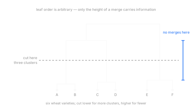
Two ideas to have in hand. A distance between two varieties is a single number for how unlike they are (the options). A dendrogram is the tree this draws: varieties along the bottom, a horizontal bar wherever two groups joined, and the bar's height telling you how far apart they were when they did.

Think of It Like This

Merging shipping companies by port distance

Forty-eight one-boat shipping companies, each in its own port. Every year the two nearest companies merge. Then the two nearest of what's left. Eventually one company owns every port, and the distance at each merger is the whole history: early ones are neighbours a few miles apart, late ones are continents joining.

Now the awkward question, and it's the entire subject. Once a company owns six ports, how far is it from another company? Measure from its closest port, its farthest, or the average across all pairs. Identical geography, genuinely different histories, and no measurement that's simply correct.

Measure from the closest port and a company creeps along a coastline one port at a time, until one firm stretches from Lisbon to Hamburg without a single jump longer than forty miles. Measure from the farthest and companies stay tight and round, chopping the coast into pieces that ignore how the ports sit.

How It Actually Works

Bottom-up, and what gets recorded

Agglomerative is the version people run. Start with 48 clusters of one variety each. Find the two closest, merge them, write down the distance they merged at. Repeat until one cluster is left. Forty-seven merges, 47 heights, and those heights are the whole output.

Because every step was kept, you choose k afterwards. Draw a horizontal line across the tree; the vertical lines it crosses count your k, and the groups below them are your clusters. Lower for more, higher for fewer, from one fitted model — which beats committing to k before you look.

Linkage is the decision that matters

"Closest" is unambiguous for two single varieties and ambiguous the moment a cluster holds more than one. The rule you pick is the linkage criterion, and it changes the answer completely.

Single linkage uses the closest pair between two clusters. It follows thin filaments, and it chains distinct groups together through any bridge of intermediate varieties.

Complete linkage uses the farthest pair. Compact round clusters, and it splits a long real group in half rather than let it stay long.

Average linkage uses the mean over all cross-pairs and sits between the two.

Ward's method uses no pair distance at all. It merges whichever two clusters raise total within-cluster variance least, making it the closest relative of k-means here, with the same taste for equal-sized blobs.

No default is right. Pick from the shape you're after, and say which you used.

Reading the tree without fooling yourself

The height of a merge is the distance at which it happened. So a long stretch of empty vertical space below a bar means those two groups had nothing in between — genuinely far apart, and that emptiness is your evidence for a cut. In the diagram, three within-family merges happen low down, then nothing for a long way, then families start joining. Cut in that empty band and you get three clusters.

Horizontal position carries no information at all. Every bar can be flipped left-to-right without changing a single merge or height, so there are billions of equally valid drawings of one tree. Two leaves drawn side by side may have joined only at the root.

And the cost is why this isn't everywhere: the distance matrix is quadratic in memory, so 48 varieties is nothing and a million rows is impossible.

Show Me the Code

Two real groups, eight stragglers strung between them, two loners. Same data, same k, two linkage rules.

1import numpy as np2
3def agglomerate(X: np.ndarray, k: int, how: str) -> list[int]:4    D = np.sqrt(((X[:, None] - X[None]) ** 2).sum(-1))5    groups: list[list[int]] = [[i] for i in range(len(X))]6    while len(groups) > k:7        pairs = [(i, j) for i in range(len(groups)) for j in range(i + 1, len(groups))]8        blocks = [D[np.ix_(groups[i], groups[j])] for i, j in pairs]9        # this cost is exactly the height the dendrogram draws the merge at10        h = [b.min() if how == "single" else b.max() for b in blocks]11        i, j = pairs[int(np.argmin(h))]12        groups[i] += groups.pop(j)13    return sorted(len(g) for g in groups)14
15rng = np.random.default_rng(1)16ends = np.vstack([rng.normal([0.0, 0.0], 0.5, (40, 2)), rng.normal([9.0, 0.0], 0.5, (40, 2))])17bridge = np.column_stack([np.linspace(1.8, 7.2, 8), np.zeros(8)])   # eight stragglers between18X = np.vstack([ends, bridge, np.column_stack([[4.5, 4.5], [9.0, 13.0]])])   # plus two loners19print("single", agglomerate(X, 3, "single"), " complete", agglomerate(X, 3, "complete"))20# -> single [1, 1, 88]  complete [2, 41, 47]

Single linkage returns 88 and two singletons. Complete linkage pairs the loners and splits the crowd near the middle. Neither is a bug.

Watch Out For

Single linkage plus a handful of in-between points

The result comes back as one cluster holding almost everything plus a few singletons, exactly as above. That shape is the signature of chaining: single linkage walked from one real group to the other across the stragglers, each hop shorter than the merge that would have kept the groups apart. Both groups are still in your data. The linkage rule refused to see the gap because the gap wasn't empty.

Look at the merge heights. Chaining shows up as a long run of merges at similar small heights, one point at a time, with no jump anywhere. Switch to average or Ward's, or strip the in-between points first — DBSCAN is built to find them, since it labels low-density points instead of assigning them.

Reading side-by-side leaves as similar

Someone points at two varieties drawn next to each other at the bottom of the tree and calls them close relatives. Look up: their branches don't join until near the root. They landed adjacent because a plotting routine had to put the leaves in some order.

Follow both leaves upward instead, find where the branches actually meet, and read that height. If you need a similarity number for two specific varieties, take it from the distance matrix, not off the picture.

The Quick Version

Every point starts as its own cluster; repeatedly merge the two closest and record the height.
The output is a tree, not a partition, so you pick k afterwards by cutting at a height.
Linkage decides the answer. Single follows filaments and chains through bridges; complete makes round clusters and splits long ones; average sits between; Ward's minimises the rise in within-cluster variance.
Merge height carries all the information. A long empty stretch below a bar is the evidence for cutting there.
Horizontal position carries none. Leaf order is arbitrary and flippable.
The distance matrix is quadratic in memory, so this doesn't scale past tens of thousands of rows.