Core ML

Learning Curves

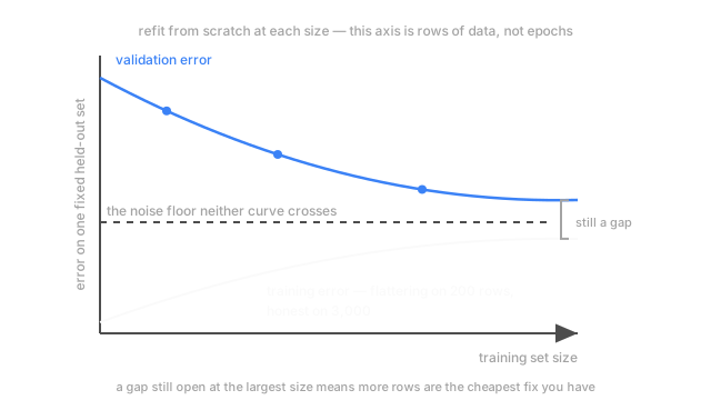
Plot error against training set size, not epochs. If both curves have flattened and the gap has closed, more data buys you nothing. That's the whole diagnosis.

Training error rises and validation error falls as you add rows, and the gap still open at the largest size is what tells you whether collecting more data would help

Why Does This Exist?

A vendor will sell you 30,000 human-judged support replies at 40 seconds of reviewer time each. That's 333 hours, most of a quarter for one person, and the question is whether the model scoring reply helpfulness from 0 to 10 gets better for it.

You can answer it with the 4,000 replies you already have, by spending less data on purpose. Fit on 200, then 400, then 800, up to 3,000, measuring each against the same held-out set. Two curves come out — error on the rows it trained on, error on the rows it didn't — and what matters isn't either level but whether they've stopped moving.

One clarification, the common mix-up. A learning curve puts training set size on the horizontal axis and refits from scratch at every size. A training curve puts optimisation steps there: one fit unrolled over time. Training curves say when to stop training, which is overfitting and underfitting. Learning curves say whether to buy more data, which no training curve can, because the data never varied.

Think of It Like This

Scooping grain to decide whether to keep scooping

Forty tonnes of wheat in a hopper, and you need its average moisture content before it's priced. Pull one scoop and test it: the answer lands in a wide range and you'd be a fool to quote it. Pull ten and average them and it settles. Pull a hundred and it barely budges.

Here's the useful part. You worked out that a hundred scoops was pointless by taking ten, plotting how the estimate moved as scoops accumulated. The flattening showed up long before you'd sampled the whole load — you never had to buy the expensive experiment to know its result.

And if the load is genuinely mixed — dry on top, damp near the outlet — no number of scoops gives you one number describing every kernel. That floor isn't a sampling problem. Telling the two cases apart is the difference between spending an afternoon and spending a quarter.

How It Actually Works

Reading the two shapes

Training error starts low and rises. With 200 rows and 40 parameters the model can fit those 200 almost exactly, so training error is flattering and meaningless. Feed it 3,000 and it can't bend around all of them, so the error climbs to the honest level. Validation error starts high and falls for the mirror reason: a fit tuned to 200 rows is partly tuned to their noise, and noise doesn't transfer.

Converged, flat, and still bad. Both curves have met, neither is moving, and the level is unacceptable. More rows are worthless — 400 to 3,000 changed nothing, and 30,000 will extend a flat line. What's left is a different model, better features, or accepting the number. The bias half of the bias-variance tradeoff reaches that from algebra instead.

A gap still wide at the largest size, validation still descending. Here more data is the cheapest thing on your list, and the only fix that costs no expressiveness. Buy the 30,000.

Why the extrapolation is honest

The gap closes on a predictable schedule. For a least-squares fit with $d$ parameters, $n$ training rows and noise variance $\sigma^2$ — the part of the target no feature explains:

\mathbb{E}[\text{training error}] \;\approx\; \sigma^2 \left( 1 - \frac{d}{n} \right)

The gap shrinks like $d/n$ . Going from 400 rows to 3,000 takes it from 0.10 to 0.013, so nearly all the remaining movement happens in the first stretch — which is why the plateau is visible at a tenth of the data you're asked to buy.

The protocol

Pick sizes spread geometrically — 200, 400, 800, 1600, 3000 — because the curvature is at the small end and even spacing wastes runs.

Refit from scratch at every size. A warm-started fit at 800 carries information from the 400-row fit, and the curve stops meaning anything.

Repeat each size on several subsamples and average, because 10 to 20 repeats is the difference between a curve and a scribble.

Hold the validation set fixed, same rows at every size — cross-validation schemes is the fallback when you can't spare a generous holdout.

And don't confuse it with a validation curve, which sweeps one hyperparameter with the dataset fixed — that answers "what setting?", not "how much data?".

Show Me the Code

Forty parameters, noise variance 4.0, and the gap closing on schedule.

1import numpy as np2
3rng = np.random.default_rng(5)4X, beta = rng.normal(size=(4000, 40)), rng.normal(size=40)5t = X @ beta + rng.normal(0.0, 2.0, 4000)    # judgement signal plus real label noise6
7
8def refit(n: int, repeats: int = 15) -> tuple[float, float]:9    r, tr, va = np.random.default_rng(n), [], []10    for _ in range(repeats):                 # small subsamples are noisy, so average11        i = r.choice(3000, n, replace=False)  # rows 3000+ stay the held-out set12        w = np.linalg.lstsq(X[i], t[i], rcond=None)[0]13        tr.append(np.mean((X[i] @ w - t[i]) ** 2))14        va.append(np.mean((X[3000:] @ w - t[3000:]) ** 2))15    return float(np.mean(tr)), float(np.mean(va))16
17
18for n in (60, 400, 3000):19    a, b = refit(n)20    print(f"n {n:5d}   train {a:6.2f}   val {b:6.2f}   gap {b - a:+6.2f}")21# -> n    60   train   1.50   val  12.46   gap +10.9622# -> n   400   train   3.67   val   4.86   gap  +1.1923# -> n  3000   train   3.97   val   4.43   gap  +0.46

At 60 rows the training error of 1.50 is a fiction and validation is three times the noise floor; read that and you'd buy data, correctly. By 400 rows the gap has fallen from 10.96 to 1.19 — 89% gone for 340 extra rows. Then 2,600 more buy 0.73, and both curves park against the 4.0 the label noise guarantees. If your plot looked like that last row, 30,000 more replies would move validation error by hundredths.

Watch Out For

Plotting against epochs and calling it a learning curve

The plot looks right. Two curves converging. Someone points at the gap, says the model is data-starved, the budget gets approved, and 30,000 replies later validation error is where it was.

The horizontal axis was training steps. Every point used all 4,000 rows, so the variable you drew a conclusion about never moved. The check is one question: did you refit from scratch at each point on the x-axis? If no, it's a training curve — right for choosing where to stop, wrong for choosing a budget.

Reading a trend off single runs at small sizes

You plot one fit per size and the curve wobbles — down at 200, up at 400, down again at 800. So you extrapolate from the last two points, and the recommendation depends on which subsample landed where.

At 200 rows the fold-to-fold spread of validation error routinely exceeds the effect you're measuring; which 200 rows you drew matters more than the fact that you drew 200. Ten to twenty repeats per size, mean and spread both plotted, and the band tells you whether the curve is still descending. It's why k-fold cross-validation beats a single split, along a second axis.

The Quick Version

The horizontal axis is training set size and you refit from scratch at every size. Epochs there is a different plot answering a different question.
Converged, flat and bad means more data is worthless. Change the model or the features.
A wide gap at the largest size with validation still falling means more data is the cheapest fix available. The gap shrinks like $d/n$ , so the plateau shows up at a fraction of what you're asked to buy.
Protocol: geometric sizes, refit from scratch, several repeats averaged per size, one fixed validation set. A single run at small sizes is a scribble.