Core ML

Pipeline Parallelism

If a model has 80 layers and you have 8 GPUs, you can put Layers 1-10 on GPU 1, and Layers 11-20 on GPU 2. GPU 1 does some math, hands the result to GPU 2, and so on. It's an assembly line for neural networks.

Why Does This Exist?

When a model is too large to fit on a single GPU, you have to split the model itself. Tensor Parallelism (TP) solves this by slicing individual matrices in half. However, TP requires massive network bandwidth because the GPUs have to synchronize multiple times per layer. This means you can generally only use TP across GPUs inside the same physical server box (connected by NVLink).

But what if you have a massive cluster of 1,000 GPUs spread across 125 different server racks? You can't use TP across standard Ethernet cables.

Pipeline Parallelism (PP) solves this. It slices the model vertically (by depth) rather than horizontally. You assign Layer 1 to Server A, and Layer 2 to Server B. Server A runs its layer, and sends a single, finalized output tensor to Server B over the network. Because communication only happens at the boundaries between layers, the network bandwidth requirement is drastically lower, allowing you to scale across thousands of servers.

Think of It Like This

Imagine an assembly line building cars. The car frame is built at Station 1. The frame is pushed to Station 2, where they add the engine. Station 2 pushes it to Station 3, where they add the doors.

Station 1 and Station 2 don't need to communicate constantly while they are working. They only communicate exactly once: when Station 1 physically hands the unfinished car to Station 2. That is Pipeline Parallelism.

How It Actually Works

In a standard, naive Pipeline Parallelism implementation (often called Inter-layer Parallelism), the model is chunked into sequential stages.

Forward Pass: The input batch of data arrives at GPU 1. GPU 1 runs Layers 1-10. It sends the output activations to GPU 2. GPU 2 runs Layers 11-20 and sends the output to GPU 3.
Backward Pass: GPU 3 calculates the loss and the gradients. It updates its weights, and sends the gradients backwards to GPU 2. GPU 2 updates, and passes the gradients backwards to GPU 1.

The Pipeline Bubble Problem

There is a fatal flaw with naive Pipeline Parallelism. While GPU 1 is processing Layer 1, GPU 2 and GPU 3 are doing absolutely nothing. They are just sitting there waiting for GPU 1 to finish. When GPU 1 finishes and hands the data to GPU 2, GPU 1 goes to sleep. In a naive implementation, only 1 GPU is active at any given time. Your hardware utilization is terrible (often $< 15\%$ ). This idle time is called the Pipeline Bubble.

The Solution: Micro-Batches (GPipe)

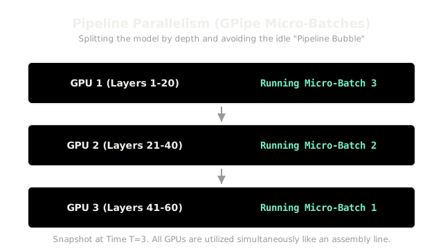
To fix the bubble, Google introduced GPipe. Instead of pushing a massive batch of 1,024 images through the pipeline all at once, you chop the batch into 16 Micro-Batches of 64 images.

GPU 1 processes Micro-Batch 1 and hands it to GPU 2.
Crucially, GPU 1 does not wait for GPU 2 to finish. GPU 1 immediately starts processing Micro-Batch 2.
By the time GPU 3 is processing Micro-Batch 1, GPU 2 is processing Micro-Batch 2, and GPU 1 is processing Micro-Batch 3.

Like a true assembly line, all stations are working simultaneously on different cars. The Pipeline Bubble is drastically reduced (though never completely eliminated, because the pipeline still has to start up and drain out at the beginning and end of every full batch).

Show Me the Code

You rarely implement the micro-batch scheduling logic yourself. Frameworks like PyTorch's torch.distributed.pipeline (or Megatron-LM) handle it. Here is the conceptual flow.

1import torch2import torch.nn as nn3from torch.distributed.pipeline.sync import Pipe4
5# 1. Define your massive sequential model6# Assume each of these blocks is a massive Transformer layer7model = nn.Sequential(8    TransformerLayer(id=1),9    TransformerLayer(id=2),10    TransformerLayer(id=3),11    TransformerLayer(id=4)12)13
14# 2. Wrap it in a Pipeline15# We assign chunks of the model to different GPUs (devices).16# Layers 1-2 go to GPU 0, Layers 3-4 go to GPU 117model = Pipe(18    model,19    chunks=8, # This is the number of Micro-Batches! (The GPipe trick)20    checkpoint="never"21)22
23# 3. Forward Pass24# The Pipe wrapper automatically chops the input batch into 8 micro-batches,25# orchestrates the asynchronous execution across GPU 0 and GPU 1,26# and reassembles the final output.27output = model(large_input_batch)28
29# 4. Backward Pass30# Automatically flows backwards through the pipeline, updating gradients.31loss = loss_fn(output, targets)32loss.backward()

Watch Out For

Memory Imbalance. In a Transformer, the first few layers usually require much more memory than the later layers because the first layer has to store the massive Embedding Matrix. If you blindly divide an 80-layer model into 4 chunks of 20 layers, GPU 1 will run out of memory (OOM) while GPU 4 is only at 50% capacity. You must manually profile the memory footprint of your model and create uneven chunks (e.g., GPU 1 gets 15 layers, GPU 2 gets 22 layers) to ensure perfectly balanced VRAM usage.

The Quick Version

Pipeline Parallelism (PP) splits a model by depth (e.g., Layers 1-10 on GPU 1, Layers 11-20 on GPU 2).
It requires very little network bandwidth compared to Tensor Parallelism, making it ideal for scaling across thousands of separate servers.
A naive pipeline leaves most GPUs idle (the Pipeline Bubble).
To fix this, the input data is chopped into Micro-Batches so all GPUs can process different slices of the data simultaneously, like an assembly line.