Core ML

Polynomial Regression

Add powers of the input as features and a straight-line model can bend into any curve — bend it too far and it memorizes noise instead of the trend.

A low-degree curve smooths through scattered points while a high-degree curve threads through every single one, wiggling wildly between them — the higher-degree fit that looks perfect on these points generalizes far worse

Why Does This Exist?

A shipping company tracks average delivery delay against distance traveled, and the relationship clearly curves — delays grow faster than distance for a while, then level off as the route optimizes. Linear regression can only draw a straight line through that curve, missing the shape entirely no matter how the line is angled.

Polynomial regression is the smallest possible fix: instead of feeding the model just distance, feed it distance, distance squared, distance cubed, and so on, and let ordinary linear regression fit coefficients to all of them at once. The model is still linear in its coefficients — nothing about the fitting procedure changes — but the curve it can draw through the data is no longer restricted to a straight line.

Think of It Like This

Bending a strip of wire to match a shape

A straight, stiff wire can only ever lie flat against a table in one direction — no amount of pushing makes it trace a curve. A wire with a few deliberate bends built in can be shaped to roughly follow a gentle curve on the table. A wire with dozens of tiny kinks, one for nearly every point on the table, can be forced to touch every single point exactly — and between those points, it zigzags wildly, tracing a shape that has nothing to do with the smooth curve the table actually suggests.

More bends means more flexibility to match what's directly in front of you, and past a certain point, that flexibility stops tracking the real shape and starts tracking every small irregularity in exactly where the points happened to land.

How It Actually Works

Turning one feature into several

Given a single input $x$ , polynomial regression of degree $d$ constructs the feature set $x, x^2, x^3, \dots, x^d$ and fits ordinary linear regression on top of it:

\hat{y} = w_0 + w_1 x + w_2 x^2 + \dots + w_d x^d

The model is called "polynomial" because of the shape of the curve it can now draw, not because the fitting method changed — the coefficients $w_0, \dots, w_d$ are still found by the same least-squares machinery linear regression uses, just applied to a wider set of columns.

Degree as a direct, visible dial on model capacity

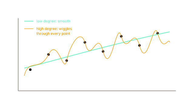
Degree 1 is ordinary linear regression: one bend allowed, none actually. Degree 2 can curve once, matching a simple parabola-shaped trend. As degree climbs, the curve gains the flexibility to bend again and again, and past a certain point — often somewhere near the number of training points itself — it gains enough flexibility to pass through every single training point exactly, leaving zero training error. This makes polynomial regression the cheapest and most visually direct way to watch overfitting and underfitting happen: the degree is a single number you can sweep, and the curve's behavior between data points is often visibly worse before any error metric confirms it.

Why zero training error can be a warning sign, not a win

A degree high enough to touch every training point has spent its flexibility fitting each point's specific noise, not the underlying trend. Between training points, the curve is free to do whatever the polynomial happens to imply, and that's typically wild oscillation, especially near the edges of the data range — a well-documented pathology called Runge's phenomenon. The curve that looks perfect on the training data is frequently the curve that generalizes worst to a new point it wasn't fit to.

Choosing degree honestly

Degree is chosen the same way any other model-complexity knob is: by comparing performance on a held-out validation set across a range of degrees, not by minimizing training error, which only ever goes down as degree rises. This is exactly the tradeoff bias–variance tradeoff formalizes — low degree underfits with high bias, high degree overfits with high variance, and the useful degree sits somewhere in between, found empirically rather than guessed.

Show Me the Code

Fitting the same noisy quadratic trend at four different polynomial degrees, and watching training and test error diverge.

1import numpy as np2
3rng = np.random.default_rng(0)4true_fn = lambda x: 0.5 * x ** 2 - x + 15x_train = np.linspace(-3, 3, 20)6y_train = true_fn(x_train) + rng.normal(0, 1.0, len(x_train))7x_test = np.linspace(-3, 3, 200)8y_test = true_fn(x_test) + rng.normal(0, 1.0, len(x_test))9
10
11def fit_poly(x: np.ndarray, y: np.ndarray, degree: int) -> np.ndarray:12    X = np.vander(x, degree + 1, increasing=True)13    w, *_ = np.linalg.lstsq(X, y, rcond=None)14    return w15
16
17def predict_poly(w: np.ndarray, x: np.ndarray) -> np.ndarray:18    return np.vander(x, len(w), increasing=True) @ w19
20
21for degree in (1, 2, 5, 15):22    w = fit_poly(x_train, y_train, degree)23    train_mse = np.mean((predict_poly(w, x_train) - y_train) ** 2)24    test_mse = np.mean((predict_poly(w, x_test) - y_test) ** 2)25    print(f"degree {degree:2d}: train MSE = {train_mse:.3f}   test MSE = {test_mse:.3f}")26# -> degree  1: train MSE = 3.846   test MSE = 2.98827# -> degree  2: train MSE = 0.592   test MSE = 1.09528# -> degree  5: train MSE = 0.368   test MSE = 1.25629# -> degree 15: train MSE = 0.139   test MSE = 5.080

Degree 2 — matching the true underlying quadratic — gets the best test error. Training error keeps dropping all the way to degree 15, exactly as expected, while test error bottoms out at degree 2 and then climbs sharply: degree 15's near-perfect training fit costs over four times the test error of the honestly-matched degree 2 model.

Watch Out For

Selecting degree by training error alone

Training error decreases monotonically as degree rises — it's mathematically guaranteed to, since more flexibility can only ever fit the training set at least as well. Choosing the degree that minimizes training error will always select the highest degree tried, regardless of how badly it generalizes. Degree selection has to come from held-out validation performance, never from the training metric directly.

Extrapolating a high-degree polynomial past the training range

A polynomial fit inside the training data's range can look entirely reasonable while diverging wildly just outside it — polynomials have no built-in reason to flatten out or stay bounded past where they were fit. Never trust a polynomial regression's predictions outside the range of x-values it was actually trained on, regardless of how good it looks inside that range.

The Quick Version

Polynomial regression fits ordinary linear regression on top of powers of the input, letting a linear method draw curved shapes.
Degree is a direct, visible dial on model capacity — low degree underfits, high degree can hit zero training error while oscillating wildly between points.
Training error decreases monotonically with degree, so it can never be used to choose degree; held-out validation error is the only honest signal.
The best degree matches the true underlying trend's complexity, not the flexibility of the model — more flexibility than the trend requires just fits noise.