Quantum Neural Networks

A quantum neural network arranges rotatable quantum gates into layered circuits analogous to deep neural networks, using classical gradient descent to steer quantum interference toward accurate predictions.

Layered Quantum Neural Network architecture showing alternating rotation blocks, entangling layers, and hybrid readout.

Why Does This Exist?

In classical deep learning, stacking linear layers with non-linear activations ( $y = \sigma(W_2 \sigma(W_1 x + b_1) + b_2)$ ) yields deep hierarchical feature extractors capable of approximating arbitrary functions. However, classical models represent data as coordinate vectors in flat Euclidean space, which scales poorly when modeling highly correlated quantum systems, molecular spin configurations, or discrete combinatorial graphs.

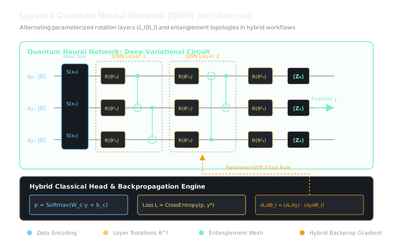
Quantum Neural Networks (QNNs) bring the structural inductive bias of deep learning—depth, repeated modular layers, and localized parameter sharing—to parameterized quantum circuits. Instead of using arbitrary unstructured quantum circuits, a QNN stacks repeated blocks of single-qubit rotation gates (analogous to linear weights) and multi-qubit entangling gates (analogous to non-linear cross-channel interactions).

By embedding a QNN into a hybrid pipeline (for example, as a quantum layer between a classical convolutional front-end and a classical classification head), machine learning practitioners harness quantum expressive capacity. Stacking unitary layers generates Fourier-like frequency components that expand exponentially with circuit depth, enabling compact networks to model complex oscillatory or topological patterns with far fewer trainable parameters than classical MLPs.

Think of It Like This

A theatrical spotlight stage with motorized polarizing color filters

Imagine an auditorium where multiple beams of colored light travel across a stage toward a screen.

Along the path of the light beams are several consecutive racks of motorized optical filters. Each filter rack represents a layer of the neural network. Within each rack, servo motors rotate individual polarizing lenses by specific angles $\theta_i$ (trainable weights). Between racks, optical prisms cross and intertwine adjacent light beams, causing them to physically overlap and interfere (entanglement).

At the back wall, light sensors measure the final color intensities and brightness at discrete spots (quantum measurement readout). A lighting director sitting in the control booth (the classical optimizer) checks whether the final stage pattern matches the desired dramatic mood. The director computes how much each filter contributed to the error, sends servo signals back to rotate each individual filter angle slightly, and repeats the test until the interference pattern is dialed in.

How It Actually Works

Layered Ansatz Construction and Hybrid Backpropagation

A Quantum Neural Network processes data through an alternating sequence of parameterized single-qubit transformations and multi-qubit entangling operations organized into $L$ discrete layers:

U(\boldsymbol{\theta}) = \prod_{l=1}^L U_l(\boldsymbol{\theta}_l)

Each layer $l$ is partitioned into two fundamental sub-blocks:

Parameterized Single-Qubit Rotations: Each qubit $q_j$ undergoes an arbitrary 3D rotation on the Bloch sphere parameterized by Euler angles $\boldsymbol{\theta}_l = (\alpha_j, \beta_j, \gamma_j)$ :

R(\alpha, \beta, \gamma) = R_z(\gamma) R_y(\beta) R_z(\alpha)

Entangling Fabric: Fixed two-qubit gates (such as CNOT or CZ) entangle adjacent qubits in a 1D chain or 2D grid. Entanglement spreads information globally across the $2^n$ -dimensional Hilbert space:

|\psi_l\rangle = W_{\text{ent}} \left( \bigotimes_{j=1}^n R(\boldsymbol{\theta}_{l, j}) \right) |\psi_{l-1}\rangle

At the output of layer $L$ , the network extracts a vector of classical continuous features $\mathbf{y} \in \mathbb{R}^k$ by measuring the expectation values of local Pauli observables $\hat{Z}_j$ :

y_j = \langle \psi(\boldsymbol{\theta}) | \hat{Z}_j | \psi(\boldsymbol{\theta}) \rangle

These quantum expectations can then be piped directly into a classical linear classification head:

\hat{p} = \text{Softmax}\left( W_{\text{class}} \mathbf{y} + b_{\text{class}} \right)

Hybrid Backpropagation via the Chain Rule

When optimizing the total cross-entropy loss $\mathcal{L}(\hat{p}, y^*)$ , gradients with respect to classical parameters ( $W_{\text{class}}, b_{\text{class}}$ ) are calculated via standard automatic differentiation. To compute gradients with respect to the internal quantum gate parameters $\theta_m$ , the system uses the multivariable chain rule:

\frac{\partial \mathcal{L}}{\partial \theta_m} = \sum_{j} \frac{\partial \mathcal{L}}{\partial y_j} \cdot \frac{\partial y_j}{\partial \theta_m}

The classical derivative $\frac{\partial \mathcal{L}}{\partial y_j}$ is supplied by PyTorch's autograd engine, while the quantum sensitivity $\frac{\partial y_j}{\partial \theta_m}$ is evaluated on the quantum processor using the parameter-shift rule:

\frac{\partial y_j}{\partial \theta_m} = \frac{1}{2} \left[ y_j\left(\theta_m + \frac{\pi}{2}\right) - y_j\left(\theta_m - \frac{\pi}{2}\right) \right]

Worked Example

Consider a 2-qubit QNN with a single parameterized layer.

Initial state: $|00\rangle = \begin{bmatrix} 1 & 0 & 0 & 0 \end{bmatrix}^\top$
Input encoding: Qubit 0 receives $x_0 = 0.0\text{ rad}$ , Qubit 1 receives $x_1 = \frac{\pi}{2}\text{ rad}$ via $R_y$ : $|\psi_0\rangle = |0\rangle \otimes \left( \cos\frac{\pi}{4}|0\rangle + \sin\frac{\pi}{4}|1\rangle \right) = \frac{1}{\sqrt{2}}|00\rangle + \frac{1}{\sqrt{2}}|01\rangle$

Step 1: Entangling Operation (CNOT) Apply CNOT with Qubit 0 as control and Qubit 1 as target: Because Qubit 0 is $|0\rangle$ in both basis terms, the target Qubit 1 is unaffected:

|\psi_1\rangle = \text{CNOT} |\psi_0\rangle = \frac{1}{\sqrt{2}}|00\rangle + \frac{1}{\sqrt{2}}|01\rangle = |0\rangle \otimes \left( \frac{1}{\sqrt{2}}|0\rangle + \frac{1}{\sqrt{2}}|1\rangle \right)

Step 2: Parameterized Rotation on Qubit 1 Apply $R_y(\theta)$ on Qubit 1 with current parameter $\theta = \frac{\pi}{2}$ : Notice that Qubit 1 is currently at angle $\frac{\pi}{2}$ . Adding another rotation of $\theta = \frac{\pi}{2}$ rotates Qubit 1 to a total angle of $\pi$ :

R_y(\pi)|0\rangle = \cos\frac{\pi}{2}|0\rangle + \sin\frac{\pi}{2}|1\rangle = 0|0\rangle + 1|1\rangle = |1\rangle

The state of the 2-qubit system becomes purely:

|\psi_{\text{final}}\rangle = |0\rangle \otimes |1\rangle = |01\rangle

Step 3: Measure Observable $\hat{Z}_1$ on Qubit 1 The Pauli-Z matrix acts as $\hat{Z}|0\rangle = +1|0\rangle$ and $\hat{Z}|1\rangle = -1|1\rangle$ . Because Qubit 1 is in state $|1\rangle$ , the expectation value is:

y = \langle \psi_{\text{final}} | \hat{Z}_1 | \psi_{\text{final}} \rangle = -1.0

Step 4: Compute Loss and Parameter Gradient Suppose our training target is $y^* = +1.0$ under mean squared error $\mathcal{L} = \frac{1}{2}(y - y^*)^2$ :

\mathcal{L} = \frac{1}{2}(-1.0 - 1.0)^2 = \frac{1}{2}(-2.0)^2 = 2.0

Classical gradient factor: $\frac{\partial \mathcal{L}}{\partial y} = y - y^* = -1.0 - 1.0 = -2.0$ . Now evaluate quantum sensitivity $\frac{\partial y}{\partial \theta}$ using parameter shifts at $\theta \pm \frac{\pi}{2}$ :

Shift up: $\theta_+ = \frac{\pi}{2} + \frac{\pi}{2} = \pi \implies \text{Total angle on Qubit 1} = \frac{\pi}{2} + \pi = \frac{3\pi}{2}$ . $\langle \hat{Z}_1 \rangle_+ = \cos(3\pi/2) = 0.0$ .
Shift down: $\theta_- = \frac{\pi}{2} - \frac{\pi}{2} = 0 \implies \text{Total angle on Qubit 1} = \frac{\pi}{2} + 0 = \frac{\pi}{2}$ . $\langle \hat{Z}_1 \rangle_- = \cos(\pi/2) = 0.0$ .
Parameter shift gradient:

\frac{\partial y}{\partial \theta} = \frac{0.0 - 0.0}{2} = 0.0

Total chain-rule gradient: $\frac{\partial \mathcal{L}}{\partial \theta} = (-2.0) \times 0.0 = 0.0$ . At $\theta = \frac{\pi}{2}$ , the expectation reaches its global minimum ( $-1.0$ ), correctly registering zero gradient slope.

Code

The following Python script simulates a 2-qubit Quantum Neural Network layer coupled with a classical loss function:

1import numpy as np2
3
4def ry(theta: float) -> np.ndarray:5    half = theta / 2.06    return np.array([7        [np.cos(half), -np.sin(half)],8        [np.sin(half),  np.cos(half)]9    ], dtype=np.complex128)10
11
12cnot = np.array([13    [1, 0, 0, 0],14    [0, 1, 0, 0],15    [0, 0, 0, 1],16    [0, 0, 1, 0]17], dtype=np.complex128)18
19z_obs = np.array([[1, 0], [0, -1]], dtype=np.complex128)20identity_2 = np.eye(2, dtype=np.complex128)21z1_observable = np.kron(identity_2, z_obs)  # I (x) Z22
23
24def forward_qnn(x_angles: list[float], theta: float) -> float:25    """Simulates 2-qubit QNN forward pass: returns expectation <Z_1>."""26    # State preparation |00>27    state = np.array([1, 0, 0, 0], dtype=np.complex128)28
29    # Input encoding: Ry(x0) (x) Ry(x1)30    enc = np.kron(ry(x_angles[0]), ry(x_angles[1]))31    state = enc @ state32
33    # Entangling layer: CNOT34    state = cnot @ state35
36    # Parameterized rotation on Qubit 1: I (x) Ry(theta)37    u_param = np.kron(identity_2, ry(theta))38    state = u_param @ state39
40    # Measurement41    exp_val = np.real(np.conj(state).T @ z1_observable @ state)42    return float(exp_val)43
44
45def hybrid_backward(x_angles: list[float], theta: float, target: float) -> tuple[float, float]:46    """Computes hybrid loss and exact chain-rule gradient dL/dtheta."""47    y = forward_qnn(x_angles, theta)48    loss = 0.5 * (y - target) ** 249    dl_dy = y - target50
51    # Parameter-shift rule for dy/dtheta52    shift = np.pi / 2.053    y_plus = forward_qnn(x_angles, theta + shift)54    y_minus = forward_qnn(x_angles, theta - shift)55    dy_dtheta = 0.5 * (y_plus - y_minus)56
57    dl_dtheta = dl_dy * dy_dtheta58    return loss, dl_dtheta59
60
61# Test parameters matching worked example62x_inputs = [0.0, np.pi / 2.0]63theta_weight = np.pi / 2.064target_y = 1.065
66loss_val, grad_val = hybrid_backward(x_inputs, theta_weight, target_y)67
68print(f"Readout y: {forward_qnn(x_inputs, theta_weight):.4f}")69# -> Readout y: -1.000070print(f"Loss: {loss_val:.4f}")71# -> Loss: 2.000072print(f"Hybrid gradient dL/dtheta: {grad_val:.4f}")73# -> Hybrid gradient dL/dtheta: 0.0000

Watch Out For

Shot noise variance corrupting classical gradient descent

On physical quantum processors, expectation values $\langle \hat{Z} \rangle$ cannot be computed analytically via statevector products. Instead, the quantum computer executes the circuit repeatedly for $N_{\text{shots}}$ runs (typically 1,000 to 10,000 shots) and computes the sample mean of binary detector clicks.

Because quantum measurement is fundamentally probabilistic, any expectation value estimate carries statistical shot noise with variance $\sigma^2 \propto \frac{1}{N_{\text{shots}}}$ . When computing the parameter-shift gradient $\frac{1}{2}(\langle M \rangle_+ - \langle M \rangle_-)$ , subtracting two noisy estimates doubles the variance. Standard classical optimizers like Adam or SGD will misinterpret this stochastic shot noise as genuine loss curvature, causing parameter updates to oscillate violently around local optima.

Fix: Never use standard vanilla SGD with fixed learning rates on physical QPUs. Employ Simultaneous Perturbation Stochastic Approximation (SPSA), which estimates gradients using random perturbations robust to shot noise, or implement adaptive shot budgeting, where the number of measurement shots dynamically increases as the optimizer approaches convergence.

The Quick Version

Quantum Neural Networks organize parameterized quantum gates into deep, layered architectures composed of rotation and entanglement stages.
The hybrid quantum-classical pipeline combines quantum circuits with classical neural networks via joint backpropagation.
The multivariable chain rule combines PyTorch classical autograd with the quantum parameter-shift rule.
Physical execution relies on finite measurement shots, requiring noise-aware optimizers like SPSA to withstand statistical measurement variance.