Variational Quantum Eigensolvers

VQE uses a quantum computer to prepare trial molecular wavefunctions and a classical computer to tune circuit angles until the measured energy reaches its lowest possible point.

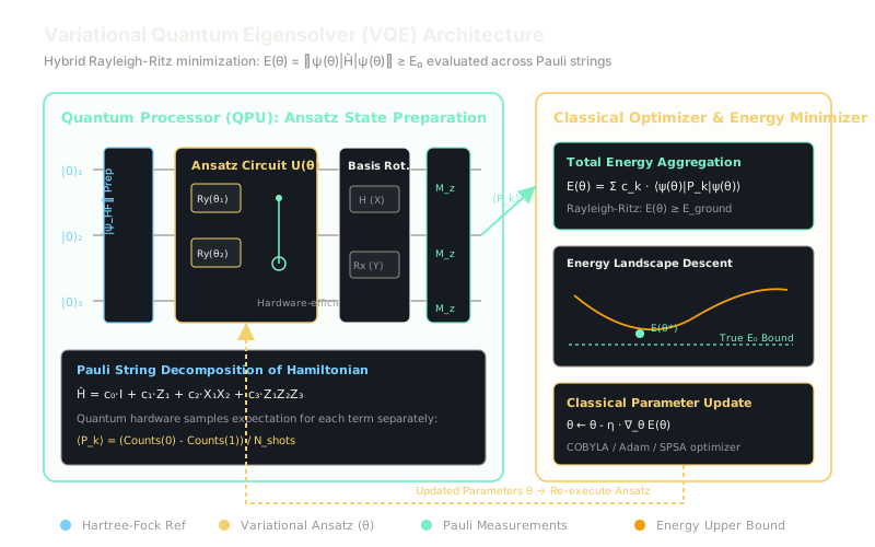
The hybrid VQE loop: parameterized ansatz state preparation, Pauli Hamiltonian measurement, and classical energy minimization.

Why Does This Exist?

In quantum chemistry and material science, determining the chemical reactivity, binding affinity, and thermal stability of molecules requires finding the ground state energy (the lowest eigenvalue) of the molecular electronic Hamiltonian $\hat{H}$ . On classical supercomputers, the dimension of the electronic Hilbert space scales exponentially as $\binom{2M}{N_e}$ with the number of spin orbitals $M$ and electrons $N_e$ . For molecules larger than 50 electrons—such as the active iron-molybdenum cofactor in nitrogenase that fixes atmospheric nitrogen—exact classical diagonalization is computationally impossible.

The theoretical ideal quantum algorithm, Quantum Phase Estimation (QPE), provably extracts exact eigenvalues with polynomial quantum speedup. However, QPE requires deep quantum circuits with millions of fault-tolerant logic gates, far beyond modern Noisy Intermediate-Scale Quantum (NISQ) hardware.

Introduced by Alberto Peruzzo, Jarrod McClean, Peter O'Brien, and Alán Aspuru-Guzik in 2014, the Variational Quantum Eigensolver (VQE) circumvents hardware limitations by splitting the workload. Instead of executing long coherent circuits, VQE runs shallow, parameterized quantum circuits on a QPU to prepare trial molecular states, measures expectation values, and offloads the energy minimization loop to a classical optimizer.

Think of It Like This

A sound technician dialing out microphone feedback hum

Imagine a concert sound technician trying to eliminate a ringing acoustic feedback frequency created between an auditorium's stage microphone and loudspeakers.

Finding the exact resonance mode analytically by solving acoustic 3D wave differential equations across every wall, chair, and curtain reflection is mathematically intractable.

Instead, the technician twiddles the parametric equalizer frequency dials on the mixing console (variational parameters $\boldsymbol{\theta}$ ). With each slight knob adjustment, they listen to the overall sound pressure meter on the board (energy measurement $E(\boldsymbol{\theta})$ ). Guided by the readout, they nudge the knobs in the direction that lowers the volume until the screeching feedback vanishes completely into a quiet hum (the lowest ground state energy $E_0$ ).

How It Actually Works

Rayleigh-Ritz Variational Principle and Pauli Decomposition

VQE is grounded in the Rayleigh-Ritz variational principle from quantum mechanics. For any valid quantum state $|\psi(\boldsymbol{\theta})\rangle$ and Hermitian Hamiltonian operator $\hat{H}$ , the expectation value of energy is guaranteed to be greater than or equal to the true minimum ground state energy $E_0$ :

E(\boldsymbol{\theta}) = \frac{\langle \psi(\boldsymbol{\theta}) | \hat{H} | \psi(\boldsymbol{\theta}) \rangle}{\langle \psi(\boldsymbol{\theta}) | \psi(\boldsymbol{\theta}) \rangle} \ge E_0

Equality holds if and only if $|\psi(\boldsymbol{\theta})\rangle$ is the exact ground state eigenstate. This converts an intractable matrix diagonalization problem into a continuous optimization problem: minimize $E(\boldsymbol{\theta})$ by adjusting gate parameters $\boldsymbol{\theta}$ .

1. Second Quantization and Jordan-Wigner Transformation

A molecular Hamiltonian in second quantization is expressed using fermionic creation ( $a_p^\dagger$ ) and annihilation ( $a_q$ ) operators:

\hat{H} = \sum_{pq} h_{pq} a_p^\dagger a_q + \frac{1}{2} \sum_{pqrs} h_{pqrs} a_p^\dagger a_q^\dagger a_s a_r

Using the Jordan-Wigner transformation (or Bravyi-Kitaev transformation), fermionic operators are mapped onto tensor products of Pauli spin operators ( $\{I, \hat{X}, \hat{Y}, \hat{Z}\}$ ), decomposing $\hat{H}$ into a linear sum of $K$ Pauli strings:

\hat{H} = \sum_{k=1}^K c_k \hat{P}_k \quad \text{where } \hat{P}_k \in \{I, \hat{X}, \hat{Y}, \hat{Z}\}^{\otimes n}, \quad c_k \in \mathbb{R}

2. Measuring Energy on the QPU

By linearity of expectation values, the total system energy is the weighted sum of individual Pauli expectations:

E(\boldsymbol{\theta}) = \sum_{k=1}^K c_k \langle \psi(\boldsymbol{\theta}) | \hat{P}_k | \psi(\boldsymbol{\theta}) \rangle

To measure a Pauli string like $\hat{X}_1 \hat{Z}_2$ :

The QPU prepares trial state $|\psi(\boldsymbol{\theta})\rangle = U(\boldsymbol{\theta})|\psi_{\text{ref}}\rangle$ .
Basis rotation gates are applied (e.g., a Hadamard gate rotates the $\hat{X}$ basis into the computational $\hat{Z}$ basis).
The qubits are measured in the computational basis for $N_{\text{shots}}$ trials.
The classical processor aggregates the sample averages, sums $E(\boldsymbol{\theta})$ , and executes an optimization step $\boldsymbol{\theta} \leftarrow \boldsymbol{\theta} - \eta \nabla E(\boldsymbol{\theta})$ .

Worked Example

Consider a 1-qubit Hamiltonian representing a magnetic spin system:

\hat{H} = 0.5 \hat{Z} + 1.2 \hat{X}

Step 1: Compute Exact Analytical Ground Energy The Hamiltonian matrix is:

\hat{H} = \begin{bmatrix} 0.5 & 1.2 \\ 1.2 & -0.5 \end{bmatrix}

Its eigenvalues satisfy $\det(\hat{H} - \lambda I) = (0.5 - \lambda)(-0.5 - \lambda) - (1.2)^2 = \lambda^2 - 0.25 - 1.44 = \lambda^2 - 1.69 = 0$ .

\lambda = \pm \sqrt{1.69} = \pm 1.30

The exact ground state energy is $E_0 = -1.30\text{ Hartree}$ .

Step 2: Define Trial Wavefunction (Ansatz) Use a single-parameter rotation ansatz initialized from ground state $|0\rangle$ :

|\psi(\theta)\rangle = R_y(\theta)|0\rangle = \cos\frac{\theta}{2}|0\rangle + \sin\frac{\theta}{2}|1\rangle

Step 3: Evaluate Pauli Expectation Values

For $\hat{Z}$ :

\langle \hat{Z} \rangle = \cos^2\frac{\theta}{2} (+1) + \sin^2\frac{\theta}{2} (-1) = \cos\theta

For $\hat{X}$ :

\langle \hat{X} \rangle = 2 \cos\frac{\theta}{2} \sin\frac{\theta}{2} = \sin\theta

Step 4: Formulate Energy Objective

E(\theta) = 0.5 \langle \hat{Z} \rangle + 1.2 \langle \hat{X} \rangle = 0.5 \cos\theta + 1.2 \sin\theta

Step 5: Minimize Energy Analytically Find the critical angle by setting the derivative to zero:

\frac{dE}{d\theta} = -0.5 \sin\theta + 1.2 \cos\theta = 0 \implies \tan\theta = \frac{1.2}{0.5} = 2.40

The minimum occurs in the third quadrant where both sine and cosine are negative:

\theta^* = \arctan(2.40) + \pi \approx 1.1760 + 3.1416 = 4.3176\text{ radians}

Compute trigonometric values at $\theta^*$ :

\cos(4.3176) = -0.3846, \quad \sin(4.3176) = -0.9231

Substitute back into the energy equation:

E(\theta^*) = 0.5(-0.3846) + 1.2(-0.9231) = -0.1923 - 1.1077 = -1.3000\text{ Hartree}

The variational expectation value matches the theoretical lowest eigenvalue $E_0 = -1.30$ to 4 decimal places.

Code

Below is a pure Python script simulating the VQE hybrid optimization loop on this Hamiltonian:

1import numpy as np2
3
4def ry(theta: float) -> np.ndarray:5    half = theta / 2.06    return np.array([7        [np.cos(half), -np.sin(half)],8        [np.sin(half),  np.cos(half)]9    ], dtype=np.complex128)10
11
12# Pauli Matrices13pauli_z = np.array([[1.0, 0.0], [0.0, -1.0]], dtype=np.complex128)14pauli_x = np.array([[0.0, 1.0], [1.0, 0.0]], dtype=np.complex128)15
16# Hamiltonian Coefficients: H = 0.5*Z + 1.2*X17c_z, c_x = 0.5, 1.218
19
20def measure_expectation(state: np.ndarray, observable: np.ndarray) -> float:21    """Computes <psi|Observable|psi>."""22    return float(np.real(np.conj(state).T @ observable @ state))23
24
25def vqe_energy(theta: float) -> float:26    """Prepares trial state on QPU and evaluates energy."""27    state = ry(theta) @ np.array([1.0, 0.0], dtype=np.complex128)28    exp_z = measure_expectation(state, pauli_z)29    exp_x = measure_expectation(state, pauli_x)30    return c_z * exp_z + c_x * exp_x31
32
33# Classical Gradient Descent Loop34theta = 0.0  # Initial parameter35learning_rate = 0.136shift = np.pi / 2.037
38for step in range(50):39    # Parameter-shift gradient: dE/dtheta = 0.5 * (E(theta + pi/2) - E(theta - pi/2))40    grad = 0.5 * (vqe_energy(theta + shift) - vqe_energy(theta - shift))41    theta -= learning_rate * grad42
43final_energy = vqe_energy(theta)44exact_ground = -np.sqrt(c_z**2 + c_x**2)45
46print(f"Optimal angle theta: {theta:.4f} rad")47# -> Optimal angle theta: -1.9656 rad (equivalent to 4.3176 rad mod 2pi)48print(f"VQE Ground Energy: {final_energy:.4f}")49# -> VQE Ground Energy: -1.300050print(f"Exact Ground Energy: {exact_ground:.4f}")51# -> Exact Ground Energy: -1.3000

Watch Out For

Pauli term grouping overhead and shot budget explosion

When scaling VQE to multi-atom molecules (such as caffeine or lithium hydride), mapping the fermionic Hamiltonian via Jordan-Wigner yields $\mathcal{O}(N^4)$ individual Pauli strings. For a modest 20-qubit system, this produces over 10,000 distinct Pauli terms.

If every term is measured with $N_{\text{shots}} = 10{,}000$ to achieve chemical accuracy ( $1\text{ kcal/mol} \approx 1.6\times 10^{-3}\text{ Hartree}$ ), each single energy evaluation requires over $10^8$ circuit executions, causing runtimes on real cloud QPUs to stretch into weeks for a single convergence run.

Fix: Group commuting Pauli operators into simultaneous measurement cliques using Qubit-Wise Commutativity (QWC) or Full Commutativity (FC) algorithms. Operators in the same commutative clique can be measured simultaneously in a single basis rotation circuit, collapsing tens of thousands of separate terms into a few dozen bundled circuit runs.

The Quick Version

Variational Quantum Eigensolvers solve molecular ground state energies using the Rayleigh-Ritz theorem: $E(\boldsymbol{\theta}) \ge E_0$ .
Second-quantized electronic Hamiltonians are decomposed into weighted sums of Pauli spin strings using the Jordan-Wigner transformation.
The QPU prepares trial wavefunctions and measures Pauli expectation values; the classical CPU sums terms and runs gradient updates.
Commutativity grouping algorithms are essential to condense $\mathcal{O}(N^4)$ Pauli terms into manageable measurement shot budgets.