Spatiotemporal Graph Neural Networks

Why Does This Exist?

Many of the most valuable real-world machine learning challenges involve networks that evolve dynamically over time: traffic congestion moving across metropolitan freeway systems, power surges propagating through electrical transmission grids, disease transmission spreading across regional flight networks, and financial liquidity flowing across banking corridors.

Traditional time-series models (like ARIMA, LSTMs, and GRUs) model temporal trends at each sensor node independently, completely ignoring the spatial physical topology connecting them; if a traffic collision halts traffic at mile marker 40, an LSTM at mile marker 39 has no mechanism to anticipate the shockwave until congestion physically reaches its sensor. Conversely, standard GNNs model static topological snapshots but lack native temporal operations. Spatiotemporal Graph Neural Networks (ST-GNNs) exist to bridge this gap: they fuse spatial graph convolutions (capturing topological diffusion across edges) with temporal models (capturing historical momentum and periodic daily trends) to forecast complex network states hours into the future.

Think of It Like This

How It Actually Works

Spatiotemporal Fusion Architectures (STGCN and DCRNN)

A spatiotemporal graph is represented as a sequence of graph signal snapshots observed over $T$ past time steps:

$\mathcal{X} = (\mathbf{X}_1, \mathbf{X}_2, \dots, \mathbf{X}_T) \in \mathbb{R}^{T \times N \times F}$

where $N$ is the number of nodes (e.g., highway sensor loops), $F$ is the feature dimension per node (e.g., speed, flow volume, occupancy), and $G = (V, E, \mathbf{W})$ is the underlying network with weighted adjacency matrix $\mathbf{W} \in \mathbb{R}^{N \times N}$. The goal is to predict the future state over the next $H$ horizon steps:

$\hat{\mathcal{Y}} = (\mathbf{X}_{T+1}, \dots, \mathbf{X}_{T+H}) \in \mathbb{R}^{H \times N \times F}$

ST-GNNs achieve this fusion through two primary paradigms:

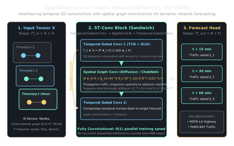
1. The Fully Convolutional Sandwich Block (STGCN)

Spatio-Temporal Graph Convolutional Networks (STGCN; Yu et al., 2018) eliminate slow, sequential recurrent loops (RNNs) in favor of a purely convolutional architecture that trains with complete temporal parallelism:

• Temporal Gated Conv (TCN): Applies 1D dilated convolutions along the time dimension across each node, followed by Gated Linear Units (GLU) to control temporal feature flow: $\mathbf{\Gamma} \star \mathbf{X} = (\mathbf{P} \star_t \mathbf{X}) \odot \sigma(\mathbf{Q} \star_t \mathbf{X})$ where $\mathbf{P}, \mathbf{Q} \in \mathbb{R}^{K_t \times F \times 2F'}$ are temporal 1D convolution kernels and $\odot$ is the Hadamard elementwise product.
• Spatial Graph Convolution: Processes the temporally filtered states using Chebyshev graph convolution or 1st-order spectral diffusion: $\mathbf{\Theta} \star_G \mathbf{H} = \mathbf{\tilde{D}}^{-1/2} \mathbf{\tilde{A}} \mathbf{\tilde{D}}^{-1/2} \mathbf{H} \mathbf{\Theta}$
• Sandwich Composition: The canonical ST-Conv block stacks: $\text{TCN} \longrightarrow \text{Spatial-GCN} \longrightarrow \text{TCN}$ surrounded by a residual skip connection $\mathbf{H}_{\text{out}} = \text{ST-Conv}(\mathbf{X}) + \mathbf{X}$.

2. Diffusion Convolutional Recurrent Neural Networks (DCRNN)

DCRNN (Li et al., 2018) replaces standard matrix multiplications in a GRU cell with Diffusion Graph Convolutions, explicitly modeling both forward downstream traffic flow and backward upstream queue spillbacks:

$\mathbf{X}_{:, j} \star_G f_\theta = \sum_{k=0}^{K-1} \left( \theta_{k, 1} \left( \mathbf{D}_O^{-1} \mathbf{W} \right)^k + \theta_{k, 2} \left( \mathbf{D}_I^{-1} \mathbf{W}^\top \right)^k \right) \mathbf{X}_{:, j}$

where $\mathbf{D}_O^{-1}\mathbf{W}$ models forward random walks (downstream flow) and $\mathbf{D}_I^{-1}\mathbf{W}^\top$ models reverse random walks (upstream congestion accumulation).

Worked Example

Consider a 2-node highway road segment: Node 1 (upstream) feeds into Node 2 (downstream) with directed transition matrix: $\mathbf{P}_{\text{fwd}} = \begin{bmatrix} 0.2 & 0.8 \\ 0.0 & 1.0 \end{bmatrix}$ where 80% of flow from Node 1 transitions to Node 2, while Node 2 has a self-loop (exit bottleneck).

Suppose we observe traffic speed over $T = 2$ past time steps for both nodes:

• Time step 1: $\mathbf{X}_1 = \begin{bmatrix} 60.0 \\ 30.0 \end{bmatrix}$ (Node 1 free flow, Node 2 slowing down).
• Time step 2: $\mathbf{X}_2 = \begin{bmatrix} 50.0 \\ 20.0 \end{bmatrix}$ (Node 1 decelerating, Node 2 gridlocked).

1. Temporal Trend (1D Convolution filter $[0.3, 0.7]$): The temporal layer weights recent observations higher: $\mathbf{H}_{\text{temp}} = 0.3 \mathbf{X}_1 + 0.7 \mathbf{X}_2$ $\mathbf{H}_{\text{temp}} = 0.3 \begin{bmatrix} 60.0 \\ 30.0 \end{bmatrix} + 0.7 \begin{bmatrix} 50.0 \\ 20.0 \end{bmatrix} = \begin{bmatrix} 18.0 + 35.0 \\ 9.0 + 14.0 \end{bmatrix} = \begin{bmatrix} 53.0 \\ 23.0 \end{bmatrix}$

2. Spatial Diffusion Convolution: Propagate spatial shockwave using forward transition matrix $\mathbf{P}_{\text{fwd}}$: $\mathbf{H}_{\text{spat}} = \mathbf{P}_{\text{fwd}} \mathbf{H}_{\text{temp}} = \begin{bmatrix} 0.2 & 0.8 \\ 0.0 & 1.0 \end{bmatrix} \begin{bmatrix} 53.0 \\ 23.0 \end{bmatrix}$ $H_{\text{spat}, 1} = (0.2 \times 53.0) + (0.8 \times 23.0) = 10.6 + 18.4 = 29.0$ $H_{\text{spat}, 2} = (0.0 \times 53.0) + (1.0 \times 23.0) = 23.0$

   Notice how Node 1's representation plummeted from $53.0$ to $29.0$: spatial diffusion immediately alerted upstream Node 1 that the downstream blockage at Node 2 will halt incoming vehicles.

Code

1from typing import Tuple2import numpy as np3
4
5class SimpleSTGCNBlock:6    """Minimal Spatiotemporal Graph Convolutional Network (ST-Conv) block."""7
8    def __init__(self, num_nodes: int, in_channels: int, out_channels: int) -> None:9        self.num_nodes = num_nodes10        rng = np.random.default_rng(seed=42)11        # 1D Temporal convolution kernel over 2 time steps12        self.w_temp: np.ndarray = rng.standard_normal((2, in_channels, out_channels)) * 0.113        # Spatial Graph convolution weight14        self.w_spat: np.ndarray = rng.standard_normal((out_channels, out_channels)) * 0.115
16    def forward(17        self,18        x: np.ndarray,          # Shape: (T=2, N, in_channels)19        norm_adj: np.ndarray,   # Shape: (N, N) normalized adjacency matrix20    ) -> np.ndarray:21        # 1. Temporal Convolution over T=2 steps22        # x[0] @ w_temp[0] + x[1] @ w_temp[1]23        t_out = x[0] @ self.w_temp[0] + x[1] @ self.w_temp[1]  # (N, out_channels)24        t_activated = np.maximum(0.0, t_out)  # ReLU25
26        # 2. Spatial Graph Convolution: A_norm @ H @ W_spat27        spat_diffused = norm_adj @ t_activated  # (N, out_channels)28        s_out = spat_diffused @ self.w_spat29        out = np.maximum(0.0, s_out)  # ReLU30        return out31
32
33# Test with 3 traffic sensors along a highway: 0 -> 1 -> 234a_norm = np.array([35    [0.5, 0.5, 0.0],36    [0.0, 0.5, 0.5],37    [0.0, 0.0, 1.0],38])39
40# Input sequence: T=2 timesteps, N=3 nodes, F=1 (speed in mph)41# Speeds slowing down over time42x_seq = np.array([43    [[65.0], [55.0], [40.0]],  # t-144    [[60.0], [45.0], [25.0]],  # t45])46
47st_block = SimpleSTGCNBlock(num_nodes=3, in_channels=1, out_channels=4)48forecast_embedding = st_block.forward(x_seq, a_norm)49print("Forecast latent embedding shape:", forecast_embedding.shape)50# -> Forecast latent embedding shape: (3, 4)51print("Sensor 0 spatial-temporal feature:", np.round(forecast_embedding[0], 4))

Watch Out For

The Quick Version

• Spatiotemporal GNNs combine spatial graph convolutions with temporal sequence modeling to forecast dynamic physical networks.
• STGCN adopts a fully convolutional sandwich structure (Temporal-Gated-Conv $\to$ Spatial-GCN $\to$ Temporal-Conv), avoiding slow sequential RNN loops.
• DCRNN uses bidirectional diffusion convolutions within GRU cells to capture downstream traffic flow and upstream queue propagation.

What to Read Next

• Neural Rendering & 3D
• Graph Embeddings
• Loss Functions