Neural Rendering & 3D

Why Does This Exist?

In traditional computer graphics, 3D scenes are modeled using discrete polygonal meshes, point clouds, or volumetric voxel grids. While highly optimized for rasterization hardware, these discrete representations present severe limitations when reconstructing real-world environments from photographs:

1. Discretization and Memory Limits: High-resolution voxel grids scale cubically as $\mathcal{O}(V^3)$; storing a fine $1024^3$ voxel grid requires gigabytes of memory, yet mostly contains empty space.
2. Non-Differentiable Rendering: Traditional triangle rasterization involves discrete rasterization boundaries (an edge is either on a pixel or off); taking derivatives of pixel colors with respect to mesh vertex coordinates produces discontinuous gradients, making end-to-end gradient descent impossible.

Neural rendering bridges computer vision and computer graphics by parameterizing 3D scenes as continuous implicit neural functions. Models like Neural Radiance Fields (NeRF; Mildenhall et al., 2020) and 3D Gaussian Splatting (Kerbl et al., 2023) use differentiable image formation models: by casting rays through virtual camera lenses and integrating light absorption mathematically, every parameter of the 3D scene can be optimized directly against raw 2D photographs using standard Adam gradient descent.

Think of It Like This

How It Actually Works

Continuous Radiance Fields and Differentiable Volume Rendering

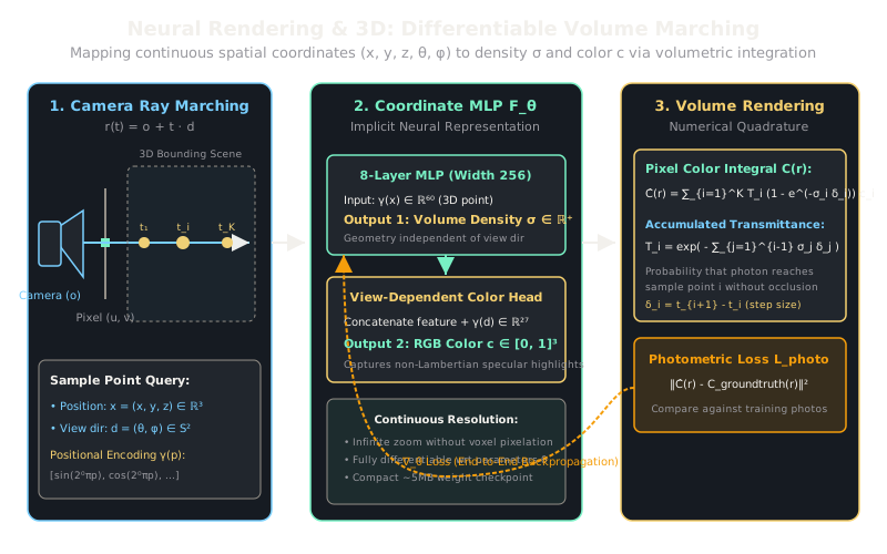
The flagship mathematical formulation of neural rendering is the Neural Radiance Field (NeRF). A 3D scene is represented as a continuous function $F_\theta: (\mathbf{x}, \mathbf{d}) \to (\mathbf{c}, \sigma)$, parameterized by a multi-layer perceptron (MLP) with weights $\theta$:

• $\mathbf{x} = (x, y, z) \in \mathbb{R}^3$ is the 3D spatial location.
• $\mathbf{d} = (\theta, \phi) \in \mathbb{S}^2$ is the 2D viewing direction vector.
• $\sigma \in \mathbb{R}^+$ is the differential volume density (how much light is absorbed/blocked at $\mathbf{x}$).
• $\mathbf{c} = (r, g, b) \in [0, 1]^3$ is the directional emitted radiance (color).

To enforce physical consistency, volume density $\sigma(\mathbf{x})$ depends strictly on spatial location $\mathbf{x}$ (geometry is view-invariant), whereas color $\mathbf{c}(\mathbf{x}, \mathbf{d})$ depends on both location and viewing angle to capture non-Lambertian effects like glossy specular reflections.

1. High-Frequency Positional Encoding

Deep neural networks exhibit a spectral bias toward learning low-frequency functions. To capture fine 3D surface textures and crisp edges, NeRF applies a sinusoidal positional encoding $\gamma: \mathbb{R} \to \mathbb{R}^{2L}$:

$\gamma(p) = \left[ \sin(2^0 \pi p), \cos(2^0 \pi p), \dots, \sin(2^{L-1} \pi p), \cos(2^{L-1} \pi p) \right]$

Setting $L = 10$ for coordinates $\mathbf{x}$ projects each spatial coordinate into a 60-dimensional frequency space.

2. Differentiable Volume Rendering (Numerical Quadrature)

For a camera ray $\mathbf{r}(t) = \mathbf{o} + t\mathbf{d}$ spanning near bound $t_n$ and far bound $t_f$, the expected color $C(\mathbf{r})$ is defined by the volume rendering integral:

$C(\mathbf{r}) = \int_{t_n}^{t_f} T(t) \sigma(\mathbf{r}(t)) \mathbf{c}(\mathbf{r}(t), \mathbf{d}) \, dt$

where $T(t) = \exp\left(-\int_{t_n}^t \sigma(\mathbf{r}(s)) \, ds\right)$ is the accumulated transmittance (the probability that the ray traverses from $t_n$ to $t$ without hitting an occluding particle).

To compute this on a GPU, the integral is discretized via stratified sampling into $K$ intervals $[t_i, t_{i+1}]$ of width $\delta_i = t_{i+1} - t_i$:

$\hat{C}(\mathbf{r}) = \sum_{i=1}^K T_i \left( 1 - \exp(-\sigma_i \delta_i) \right) \mathbf{c}_i$

$T_i = \exp\left( -\sum_{j=1}^{i-1} \sigma_j \delta_j \right)$

Because every operation in this summation is smooth and differentiable with respect to $\sigma_i$ and $\mathbf{c}_i$, the photometric reconstruction loss:

$\mathcal{L} = \sum_{\mathbf{r} \in \mathcal{R}} \left\| \hat{C}(\mathbf{r}) - C_{\text{groundtruth}}(\mathbf{r}) \right\|_2^2$

propagates exact analytical gradients back to the weights $\theta$ of the MLP without needing 3D supervision, depth sensors, or surface meshes.

Worked Example

Consider a single camera ray sampled at $K = 2$ intervals with uniform step size $\delta_1 = \delta_2 = 1.0$:

• Sample 1: Volume density $\sigma_1 = 0.5$, Color $\mathbf{c}_1 = [1.0, 0.0, 0.0]$ (pure red).
• Sample 2: Volume density $\sigma_2 = 2.0$, Color $\mathbf{c}_2 = [0.0, 1.0, 0.0]$ (pure green).

1. Calculate Sample 1 Transmittance and Alpha:

   • Transmittance $T_1 = \exp(0) = 1.0$ (no obstruction prior to sample 1).
   • Absorption probability $\alpha_1 = 1 - \exp(-\sigma_1 \delta_1) = 1 - \exp(-0.5) \approx 1 - 0.6065 = 0.3935$.
   • Contribution of sample 1: $\mathbf{C}_1 = T_1 \alpha_1 \mathbf{c}_1 = 1.0 \times 0.3935 \times [1.0, 0.0, 0.0] = [0.3935, 0.0, 0.0]$

2. Calculate Sample 2 Transmittance and Alpha:

   • Transmittance $T_2 = \exp(-\sigma_1 \delta_1) = \exp(-0.5) \approx 0.6065$ (only 60.6% of light penetrates past sample 1).
   • Absorption probability $\alpha_2 = 1 - \exp(-\sigma_2 \delta_2) = 1 - \exp(-2.0) \approx 1 - 0.1353 = 0.8647$.
   • Contribution of sample 2: $\mathbf{C}_2 = T_2 \alpha_2 \mathbf{c}_2 = 0.6065 \times 0.8647 \times [0.0, 1.0, 0.0] \approx 0.5244 \times [0.0, 1.0, 0.0] = [0.0, 0.5244, 0.0]$

3. Total Pixel Color: $\hat{C}(\mathbf{r}) = \mathbf{C}_1 + \mathbf{C}_2 = [0.3935, 0.5244, 0.0]$ The pixel reflects a blend of both layers, with the denser background layer partially occluded by the semi-transparent foreground fog.

Code

1import numpy as np2
3
4def volume_render_ray(5    densities: np.ndarray,  # Shape: (K,) volume densities sigma >= 06    colors: np.ndarray,     # Shape: (K, 3) RGB colors in [0, 1]7    step_sizes: np.ndarray, # Shape: (K,) delta distances between sample points8) -> np.ndarray:9    """Discretized differentiable volume rendering via numerical quadrature."""10    k = densities.shape[0]11
12    # 1. Opacity for each sample interval: alpha_i = 1 - exp(-sigma_i * delta_i)13    sigmas_deltas = densities * step_sizes14    alphas = 1.0 - np.exp(-sigmas_deltas)15
16    # 2. Accumulated transmittance: T_i = exp(-sum_{j=1}^{i-1} sigma_j * delta_j)17    # Cumulative sum with 0 prepended for T_1 = 1.018    accumulated_optical_depth = np.cumsum(sigmas_deltas)19    transmittance = np.ones(k, dtype=np.float64)20    transmittance[1:] = np.exp(-accumulated_optical_depth[:-1])21
22    # 3. Composite sample weights: w_i = T_i * alpha_i23    weights = transmittance * alphas24
25    # 4. Integrate pixel color: C = sum(weights * colors)26    pixel_color = np.sum(weights[:, np.newaxis] * colors, axis=0)27    return pixel_color28
29
30# Test with 2 sample points31dens = np.array([0.5, 2.0])32cols = np.array([33    [1.0, 0.0, 0.0],  # Red foreground34    [0.0, 1.0, 0.0],  # Green background35])36deltas = np.array([1.0, 1.0])37
38rendered_pixel = volume_render_ray(dens, cols, deltas)39print("Rendered RGB Pixel:", np.round(rendered_pixel, 4))40# -> Rendered RGB Pixel: [0.3935 0.5245 0.    ]

Watch Out For

The Quick Version

• Neural rendering represents continuous 3D geometry and view-dependent color using neural networks optimized end-to-end via 2D photometric loss.
• High-frequency sinusoidal positional encodings overcome the spectral bias of MLPs, preserving crisp textures and sharp surface boundaries.
• Volume rendering uses numerical quadrature to integrate transmittance and opacity along camera rays in a fully differentiable pipeline.

What to Read Next

• Graph Embeddings
• DeepWalk and Node2Vec
• Backpropagation