Graph Embeddings

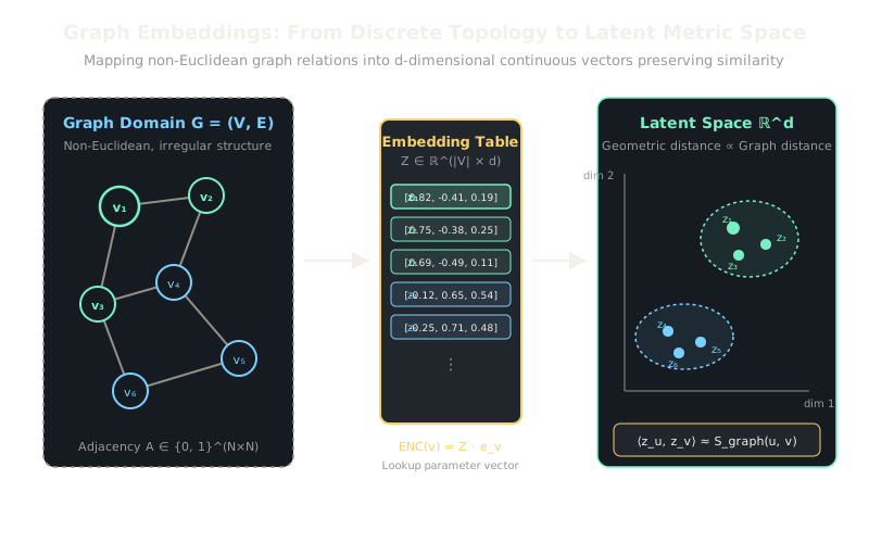
Why Does This Exist?

Standard machine learning models like linear classifiers, gradient-boosted trees, and multi-layer perceptrons expect inputs formatted as rigid, fixed-dimensional feature vectors in Euclidean space $\mathbb{R}^d$. Real-world relational datasets—such as financial transaction trails, citation graphs, protein interactomes, and social networks—are fundamentally non-Euclidean: each entity has an arbitrary number of connections, unordered neighbors, and complex multihop dependencies.

Representing a graph of $N$ nodes naively via its adjacency matrix $A \in \{0, 1\}^{N \times N}$ leads to catastrophic failure at scale. An adjacency row for a node is extremely high-dimensional, sparse (often over 99.9% zeros), and brittle: reordering node indices completely shuffles the vector, and the dot product between two disconnected nodes sharing a mutual neighbor evaluates to zero. Graph embeddings solve this disconnect by projecting discrete nodes, edges, or entire subgraphs into a compact, low-dimensional coordinate space $\mathbb{R}^d$ ($d \ll N$, often 64 to 256) where geometric operations like the dot product directly reflect topological proximity and structural equivalence.

Think of It Like This

How It Actually Works

The Encoder-Decoder Framework

The universal formulation of node-level graph embeddings operates through an encoder-decoder framework. Given a graph $G = (V, E)$, the encoder function $\text{ENC}: V \to \mathbb{R}^d$ maps each node $u \in V$ to a low-dimensional vector $\mathbf{z}_u \in \mathbb{R}^d$.

In shallow (transductive) embedding algorithms, the encoder is simply an embedding lookup table parameterized by a matrix $\mathbf{Z} \in \mathbb{R}^{|V| \times d}$, such that:

$\text{ENC}(u) = \mathbf{Z} \mathbf{e}_u = \mathbf{z}_u$

where $\mathbf{e}_u \in \{0, 1\}^{|V|}$ is an indicator one-hot vector for node $u$.

The decoder function $\text{DEC}: \mathbb{R}^d \times \mathbb{R}^d \to \mathbb{R}$ reconstructs pairwise relational similarity between nodes from their coordinate representations. The most common decoder is the inner product:

$\text{DEC}(\mathbf{z}_u, \mathbf{z}_v) = \mathbf{z}_u^\top \mathbf{z}_v$

The training objective minimizes empirical discrepancy between the decoded vector proximity and a pre-defined graph similarity metric $S_G(u, v)$ over all node pairs:

$\mathcal{L} = \sum_{u, v \in V} \ell\left(\text{DEC}(\mathbf{z}_u, \mathbf{z}_v), S_G(u, v)\right)$

Depending on the definition of $S_G(u, v)$:

• First-order proximity sets $S_G(u, v) = A_{uv}$, penalizing coordinates if immediate neighbors do not share a large dot product.
• Second-order proximity enforces that nodes sharing similar neighborhood probability distributions $p(\cdot | u) \approx p(\cdot | v)$ have nearby coordinates, even if no direct edge exists between $u$ and $v$.
• High-order random walk proximity samples random walks to maximize the log-probability of co-occurrence within a temporal context window.

Worked Example

Consider a small 4-node undirected graph with edges $(1, 2)$, $(1, 3)$, and $(3, 4)$. We train a 2-dimensional embedding ($d = 2$) using a dot-product decoder and a sigmoid cross-entropy loss with negative sampling.

Let the current embeddings be:

• $\mathbf{z}_1 = [0.8, 0.2]^\top$
• $\mathbf{z}_2 = [0.6, 0.4]^\top$
• $\mathbf{z}_3 = [0.7, -0.1]^\top$
• $\mathbf{z}_4 = [-0.5, 0.5]^\top$

We compute the loss for a true positive edge $(1, 2)$ and a sampled negative edge $(1, 4)$ (nodes 1 and 4 have no direct connection):

1. Positive Pair $(1, 2)$: The inner product is: $\mathbf{z}_1^\top \mathbf{z}_2 = (0.8 \times 0.6) + (0.2 \times 0.4) = 0.48 + 0.08 = 0.56$ The predicted edge probability is: $\sigma(\mathbf{z}_1^\top \mathbf{z}_2) = \frac{1}{1 + e^{-0.56}} \approx \frac{1}{1 + 0.5712} \approx 0.6364$ The positive loss contribution is: $\mathcal{L}_{\text{pos}} = -\log(0.6364) \approx 0.4519$

2. Negative Pair $(1, 4)$: The inner product is: $\mathbf{z}_1^\top \mathbf{z}_4 = (0.8 \times -0.5) + (0.2 \times 0.5) = -0.40 + 0.10 = -0.30$ The negative probability is: $\sigma(-\mathbf{z}_1^\top \mathbf{z}_4) = \sigma(0.30) = \frac{1}{1 + e^{-0.30}} \approx \frac{1}{1 + 0.7408} \approx 0.5744$ The negative loss contribution is: $\mathcal{L}_{\text{neg}} = -\log(0.5744) \approx 0.5544$

3. Total Pairwise Loss: $\mathcal{L} = \mathcal{L}_{\text{pos}} + \mathcal{L}_{\text{neg}} = 0.4519 + 0.5544 = 1.0063$

4. Gradient Update for $\mathbf{z}_1$: The gradient with respect to $\mathbf{z}_1$ evaluates to: $\frac{\partial \mathcal{L}}{\partial \mathbf{z}_1} = (\sigma(\mathbf{z}_1^\top \mathbf{z}_2) - 1)\mathbf{z}_2 + \sigma(\mathbf{z}_1^\top \mathbf{z}_4)\mathbf{z}_4$ $\frac{\partial \mathcal{L}}{\partial \mathbf{z}_1} = (0.6364 - 1)\begin{bmatrix} 0.6 \\ 0.4 \end{bmatrix} + (1 - 0.5744)\begin{bmatrix} -0.5 \\ 0.5 \end{bmatrix}$ $\frac{\partial \mathcal{L}}{\partial \mathbf{z}_1} = -0.3636 \begin{bmatrix} 0.6 \\ 0.4 \end{bmatrix} + 0.4256 \begin{bmatrix} -0.5 \\ 0.5 \end{bmatrix} = \begin{bmatrix} -0.2182 - 0.2128 \\ -0.1454 + 0.2128 \end{bmatrix} = \begin{bmatrix} -0.4310 \\ 0.0674 \end{bmatrix}$ Using learning rate $\eta = 0.1$, the updated coordinate is: $\mathbf{z}_1 \leftarrow \begin{bmatrix} 0.8 \\ 0.2 \end{bmatrix} - 0.1 \begin{bmatrix} -0.4310 \\ 0.0674 \end{bmatrix} = \begin{bmatrix} 0.8431 \\ 0.1933 \end{bmatrix}$ Node 1 moved closer to its true neighbor node 2 along dimension 0.

Code

1import numpy as np2
3
4class ShallowGraphEmbedding:5    """Matrix-factorization style shallow node embedding table."""6
7    def __init__(self, num_nodes: int, embedding_dim: int, lr: float = 0.05) -> None:8        self.num_nodes = num_nodes9        self.embedding_dim = embedding_dim10        self.lr = lr11        # Initialize embedding table with small Gaussian noise12        rng = np.random.default_rng(seed=42)13        self.embeddings: np.ndarray = rng.standard_normal((num_nodes, embedding_dim)) * 0.114
15    def _sigmoid(self, x: float) -> float:16        return float(1.0 / (1.0 + np.exp(-np.clip(x, -15.0, 15.0))))17
18    def train_step(self, u: int, v_pos: int, v_neg: int) -> float:19        """Single SGD step optimizing positive edge (u, v_pos) against negative pair (u, v_neg)."""20        z_u = self.embeddings[u]21        z_pos = self.embeddings[v_pos]22        z_neg = self.embeddings[v_neg]23
24        # Forward passes25        dot_pos = float(np.dot(z_u, z_pos))26        dot_neg = float(np.dot(z_u, z_neg))27
28        p_pos = self._sigmoid(dot_pos)29        p_neg = self._sigmoid(dot_neg)30
31        loss = -np.log(max(p_pos, 1e-7)) - np.log(max(1.0 - p_neg, 1e-7))32
33        # Gradient derivations34        grad_u = (p_pos - 1.0) * z_pos + p_neg * z_neg35        grad_pos = (p_pos - 1.0) * z_u36        grad_neg = p_neg * z_u37
38        # In-place parameter updates39        self.embeddings[u] -= self.lr * grad_u40        self.embeddings[v_pos] -= self.lr * grad_pos41        self.embeddings[v_neg] -= self.lr * grad_neg42
43        return float(loss)44
45
46# Verify execution47model = ShallowGraphEmbedding(num_nodes=4, embedding_dim=2, lr=0.1)48initial_loss = model.train_step(u=0, v_pos=1, v_neg=3)49# -> initial_loss around 1.386350updated_sim = float(np.dot(model.embeddings[0], model.embeddings[1]))51# -> similarity increases between connected nodes52print(f"Initial loss: {initial_loss:.4f}, Connected dot product: {updated_sim:.4f}")

Watch Out For

The Quick Version

• Graph embeddings map discrete, non-Euclidean graph topologies into compact, continuous vectors where Euclidean distances or dot products reflect network proximity.
• The encoder-decoder paradigm abstracts graph embeddings into an encoder that extracts coordinates and a decoder that reconstructs pairwise edge affinities.
• Shallow lookups optimize an explicit parameter vector per node, which is computationally fast for static networks but cannot generalize inductively to unseen nodes.

What to Read Next

• DeepWalk and Node2Vec
• Message Passing Neural Networks
• Gradient Descent