Quantum Machine Learning

Classical machine learning maps data into vectors in flat coordinate spaces, while quantum machine learning maps numbers into quantum wave amplitudes where entanglement and interference reveal complex patterns.

Quantum feature encoding, parameterized unitary rotation gates, entanglement, and measurement yielding classical expectation values.

Why Does This Exist?

Support Vector Machines and kernel methods revolutionized classical machine learning by applying the "kernel trick": implicitly projecting $d$ -dimensional feature vectors $x$ into a high-dimensional feature space $\Phi(x)$ where non-linear boundaries become linearly separable. However, classical computers struggle with kernels whose inner products require integrating over astronomical state spaces; evaluating certain kernel matrices takes exponential time $\mathcal{O}(2^d)$ .

Quantum Machine Learning (QML) bridges quantum mechanics and statistical learning. A quantum processor with $n$ qubits operates natively in a $2^n$ -dimensional complex Hilbert space $\mathcal{H} = \mathbb{C}^{2^n}$ . For a mere 50 qubits, the state space exceeds $10^{15}$ complex dimensions—larger than the memory capacity of any classical supercomputer.

By encoding classical data vectors into quantum states via unitary transformations $|\Phi(x)\rangle = U_\Phi(x)|0\rangle^{\otimes n}$ , quantum circuits can calculate inner products $k(x, x') = |\langle \Phi(x) | \Phi(x') \rangle|^2$ and execute variational optimizations across high-dimensional geometries. Rather than waiting for fault-tolerant quantum mainframes, modern QML focuses on hybrid quantum-classical algorithms that run short-depth circuits on noisy intermediate-scale quantum (NISQ) devices, offloading parameter updates to classical gradient optimizers.

Think of It Like This

An optical laser interferometer measuring microscopic film contours

Imagine trying to inspect an invisible, uneven microscopic grease film smeared on a pane of glass.

A classical machine learning approach is using a mechanical micrometer needle to physically touch the glass at 10,000 grid points. Computing the global contour from individual mechanical touch points requires dense measurements, slow sweeps, and massive matrix calculations.

A quantum machine learning approach is shining a coherent laser beam through the glass. The light wave naturally splits, passes through the grease layer at speed, and recombines on a detector screen. The physical wave properties of the light—phase shifts, wave interference, and constructive ripple fringes—instantly integrate the entire surface topography into a visible interference pattern. The quantum system does not simulate the high-dimensional geometry; its physical quantum states embody the geometry directly.

How It Actually Works

Quantum Feature Maps and Parameterized Unitary Circuits

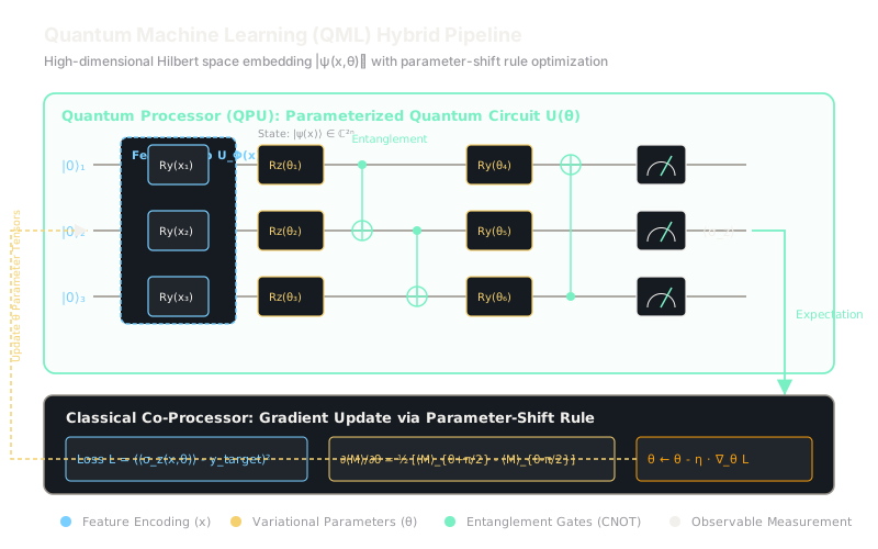
A typical hybrid QML pipeline executes in three sequential stages:

Quantum Feature Encoding ( $U_\Phi(x)$ ): Classical features $x = [x_1, \dots, x_n]^\top$ are encoded into an $n$ -qubit quantum state. In angle encoding, each classical feature rotates a qubit around the Bloch sphere using a single-qubit Pauli rotation gate:

|\Phi(x)\rangle = \bigotimes_{j=1}^n R_y(x_j) |0\rangle^{\otimes n} = \bigotimes_{j=1}^n \left( \cos\frac{x_j}{2} |0\rangle + \sin\frac{x_j}{2} |1\rangle \right)

Parameterized Variational Circuit ( $U(\theta)$ ): The encoded state is transformed by an ansatz circuit composed of trainable rotation gates $R_y(\theta_k), R_z(\theta_k)$ and entangling operations (such as Controlled-NOT or CNOT gates):

|\psi(x, \theta)\rangle = U(\theta) |\Phi(x)\rangle = \left( \prod_{l=1}^L U_l(\theta_l) W_{\text{ent}} \right) |\Phi(x)\rangle

Entanglement creates non-local quantum correlations between qubits, transforming product states into superpositions that have no classical factorized representation.

Measurement and the Parameter-Shift Rule: The output prediction is the expectation value of an observable operator $\hat{M}$ (such as Pauli-Z $\hat{\sigma}_z$ ):

y_{\text{pred}}(x, \theta) = \langle \psi(x, \theta) | \hat{M} | \psi(x, \theta)\rangle

Because quantum hardware outputs probabilistic projective measurement counts rather than analytical equations, standard backpropagation cannot inspect intermediate circuit states without collapsing the wave function. Instead, gradients are evaluated exactly using the parameter-shift rule:

\frac{\partial \langle \hat{M} \rangle}{\partial \theta_k} = \frac{1}{2} \left[ \langle \hat{M} \rangle_{\theta_k + \frac{\pi}{2}} - \langle \hat{M} \rangle_{\theta_k - \frac{\pi}{2}} \right]

This remarkable identity proves that evaluating the circuit at two macroscopic angle offsets $\pm \frac{\pi}{2}$ yields the exact analytical gradient of the quantum expectation with respect to parameter $\theta_k$ .

Worked Example

Let us trace a single-qubit quantum classifier ( $n=1$ ) evaluating an input feature $x$ and trainable weight $\theta$ .

Input feature: $x = 0.5\text{ radians}$
Trainable parameter: $\theta = 0.8\text{ radians}$
Measurement operator: Pauli-Z observable $\hat{\sigma}_z = \begin{bmatrix} 1 & 0 \\ 0 & -1 \end{bmatrix}$

Step 1: Quantum State Preparation Rotate initial ground state $|0\rangle = \begin{bmatrix} 1 \\ 0 \end{bmatrix}$ by input angle $x$ via $R_y(x)$ :

R_y(x) = \begin{bmatrix} \cos(x/2) & -\sin(x/2) \\ \sin(x/2) & \cos(x/2) \end{bmatrix} = \begin{bmatrix} \cos(0.25) & -\sin(0.25) \\ \sin(0.25) & \cos(0.25) \end{bmatrix} \approx \begin{bmatrix} 0.9689 & -0.2474 \\ 0.2474 & 0.9689 \end{bmatrix}

|\Phi(x)\rangle = R_y(0.5)|0\rangle \approx 0.9689 |0\rangle + 0.2474 |1\rangle

Step 2: Apply Parameterized Ansatz $R_y(\theta)$ Because rotations around the same axis commute, the total rotation angle is simply $\alpha = x + \theta = 0.5 + 0.8 = 1.3\text{ radians}$ :

|\psi(x, \theta)\rangle = R_y(1.3)|0\rangle = \cos(0.65)|0\rangle + \sin(0.65)|1\rangle \approx 0.7961 |0\rangle + 0.6052 |1\rangle

Step 3: Measure Expectation Value $\langle \hat{\sigma}_z \rangle$

\langle \hat{\sigma}_z \rangle = \langle \psi | \hat{\sigma}_z | \psi \rangle = |\cos(0.65)|^2 \times (+1) + |\sin(0.65)|^2 \times (-1)

\langle \hat{\sigma}_z \rangle = (0.7961)^2 - (0.6052)^2 = 0.6338 - 0.3662 = +0.2676

Analytical check: $\cos(x + \theta) = \cos(1.3) \approx 0.2675$ .

Step 4: Gradient via Parameter-Shift Rule Evaluate the circuit at $\theta + \pi/2$ and $\theta - \pi/2$ :

Forward shift: $\theta_+ = 0.8 + 1.5708 = 2.3708 \implies \alpha_+ = 0.5 + 2.3708 = 2.8708\text{ rad}$ . $\langle \hat{\sigma}_z \rangle_+ = \cos(2.8708) \approx -0.9684$ .
Backward shift: $\theta_- = 0.8 - 1.5708 = -0.7708 \implies \alpha_- = 0.5 - 0.7708 = -0.2708\text{ rad}$ . $\langle \hat{\sigma}_z \rangle_- = \cos(-0.2708) \approx +0.9636$ .
Compute gradient:

\frac{\partial \langle \hat{\sigma}_z \rangle}{\partial \theta} = \frac{-0.9684 - (+0.9636)}{2} = \frac{-1.9320}{2} = -0.9660

Direct calculus check: $\frac{d}{d\theta}[\cos(x + \theta)] = -\sin(1.3) = -0.9636$ . The parameter shift reproduces the true analytical derivative with zero numerical finite-difference approximation errors.

Code

Below is a pure Python and NumPy simulation of a hybrid quantum machine learning step demonstrating feature encoding and the parameter-shift rule:

1import numpy as np2
3
4def ry_gate(angle: float) -> np.ndarray:5    """Returns 2x2 unitary rotation matrix Ry(angle)."""6    half = angle / 2.07    return np.array([8        [np.cos(half), -np.sin(half)],9        [np.sin(half),  np.cos(half)]10    ], dtype=np.complex128)11
12
13def run_qml_circuit(x: float, theta: float) -> float:14    """Executes state preparation and parameterized rotation, returning <sigma_z>."""15    # Ground state |0>16    state = np.array([1.0, 0.0], dtype=np.complex128)17
18    # Unitary evolution: U(theta) @ U_Phi(x) @ |0>19    u_feat = ry_gate(x)20    u_param = ry_gate(theta)21    final_state = u_param @ (u_feat @ state)22
23    # Observable sigma_z = diag(1, -1)24    sigma_z = np.array([[1.0, 0.0], [0.0, -1.0]], dtype=np.complex128)25    exp_val = np.real(np.conj(final_state).T @ sigma_z @ final_state)26    return float(exp_val)27
28
29def parameter_shift_gradient(x: float, theta: float) -> float:30    """Computes exact gradient using the parameter-shift rule."""31    shift = np.pi / 2.032    forward_eval = run_qml_circuit(x, theta + shift)33    backward_eval = run_qml_circuit(x, theta - shift)34    return 0.5 * (forward_eval - backward_eval)35
36
37# Verification test matching worked example38x_val = 0.539theta_val = 0.840
41exp_z = run_qml_circuit(x_val, theta_val)42grad_theta = parameter_shift_gradient(x_val, theta_val)43
44print(f"Expectation <sigma_z>: {exp_z:.4f}")45# -> Expectation <sigma_z>: 0.267546print(f"Parameter-shift Gradient: {grad_theta:.4f}")47# -> Parameter-shift Gradient: -0.9636

Watch Out For

Barren plateaus in deep random quantum ansatz circuits

When scaling parameterized quantum circuits to many qubits ( $n > 20$ ), practitioners frequently encounter barren plateaus. As proven by McClean et al., if the ansatz circuit has random initialization or deep entangling layers that form an approximate 2-design over the unitary group, the variance of the gradient across parameter space vanishes exponentially:

\text{Var}\left[ \frac{\partial \langle \hat{M} \rangle}{\partial \theta_k} \right] \in \mathcal{O}\left( \frac{1}{2^n} \right)

The loss landscape becomes almost perfectly flat in every direction. Standard gradient descent requires an exponential number of quantum measurement shots to distinguish true gradient signal from quantum shot noise.

Fix: Never initialize deep variational circuits with uniform random parameters. Use identity-initialized circuits (where gates initially compose to the identity), design shallow local cost functions (measuring single-qubit observables rather than global multi-qubit operators), or implement problem-inspired architectures like Quantum Convolutional Neural Networks (QCNNs) that provably avoid barren plateaus.

The Quick Version

Quantum Machine Learning maps classical data into the amplitudes of high-dimensional complex Hilbert spaces ( $2^n$ dimensions for $n$ qubits).
Hybrid quantum-classical pipelines evaluate parameterized unitary circuits on QPUs while offloading gradient updates to classical CPUs.
The parameter-shift rule allows hardware to calculate exact analytical gradients by evaluating circuits at $\pm \frac{\pi}{2}$ angle offsets.
Deep random ansatzes suffer from barren plateaus, where gradients vanish exponentially unless mitigated by shallow circuits and local observables.