Core ML

State Space Models

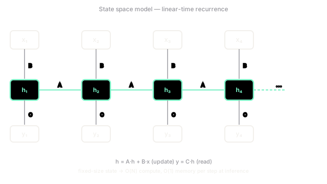
A state space model compresses the entire past into a fixed-size hidden state that is updated one input at a time, giving linear-time inference without the quadratic score matrix that attention requires.

A state space model compresses all past inputs into a fixed-size hidden state h that is updated each step using learned matrices A and B; the output is read from the state via C, giving linear-time inference with no attention score matrix

Why Does This Exist?

The attention complexity problem is real: every token attending to every other token gives $O(N^2)$ compute. Linear attention approximates softmax with a kernel to get $O(N)$ , but pays in quality. A completely different family of models — state space models — achieves $O(N)$ at training and $O(1)$ per step at inference by never computing pairwise scores at all.

SSMs come from control theory, not deep learning. The core idea is a linear dynamical system: a hidden state $h$ that is updated according to a transition matrix $A$ each time a new input $x$ arrives, plus an input matrix $B$ that injects the new input into the state, and an output matrix $C$ that reads the output $y$ from the state:

h_t = A h_{t-1} + B x_t, \quad y_t = C h_t

The state $h$ is the model's compressed memory. At inference, generating the next token costs $O(d^2)$ — one matrix multiply to update the state, one to read the output — regardless of how many tokens came before. That's the hardware win: O(1) memory and O(1) compute per step.

Gu et al. formalised this as the Structured State Space Sequence Model (S4) in 2021, showing that with a carefully chosen HiPPO initialisation for $A$ , the model could capture long-range dependencies that RNNs and truncated attention both miss.

Think of It Like This

A rolling stock ticker versus a full trade history

A financial dashboard showing a rolling average doesn't store every trade ever made. It maintains a compact running summary — the current mean, variance, trend — and updates that summary as each new trade arrives. The summary has fixed size no matter how many trades have passed. Looking up "the trend" costs one read of the summary, not a scan of the history.

An SSM is that rolling summary, but learned. The state matrix $A$ determines how the summary decays and evolves; $B$ determines how new inputs modify it; $C$ determines what to extract. At inference, generating a token costs one update and one read — no scan.

How It Actually Works

The discretisation step

Continuous-time SSMs are defined with differential equations. To use them on discrete sequences (tokens, not audio samples in continuous time), the continuous matrices $A$ and $B$ are discretised to obtain a discrete-time recurrence using a zero-order hold or bilinear method. The result is a set of discrete matrices $\bar{A}$ and $\bar{B}$ that depend on a learned step size $\Delta$ :

\bar{A} = \exp(\Delta A), \quad \bar{B} = (\bar{A} - I) A^{-1} B \approx \Delta B

Training efficiency: the convolutional view

During training, you have all tokens at once, so you can compute the SSM as a convolution rather than a recurrence. The state unrolled over time gives a response $y = x * K$ where $K$ is the SSM's impulse response (a vector of length $N$ ). Computing a convolution of two $N$ -vectors costs $O(N \log N)$ via FFT — competitive with attention for many sequence lengths.

The two views — recurrent for inference, convolutional for training — are mathematically equivalent given the same $A$ , $B$ , $C$ . The model trains efficiently and infers efficiently.

The HiPPO initialisation

The choice of $A$ matters a lot. Random $A$ typically leads to vanishing/exploding gradients, just as in RNNs. HiPPO (High-Order Polynomial Projection Operators) initialises $A$ to be a matrix that theoretically compresses the past optimally — projecting the input history onto a family of orthogonal polynomials. In practice this means the model starts with a good inductive bias for long-range dependencies, rather than having to learn that from scratch.

Show Me the Code

Running a tiny SSM recurrence and verifying the output matches the equivalent convolution.

1import numpy as np2
3rng = np.random.default_rng(9)4n, d = 16, 4   # sequence length, state dimension5
6A = 0.9 * np.eye(d)          # simple stable diagonal A7B = rng.standard_normal((d, 1)) * 0.18C = rng.standard_normal((1, d)) * 0.19x = rng.standard_normal((n, 1))   # input sequence10
11# Recurrent form (inference mode)12h = np.zeros(d)13y_rec = np.zeros(n)14for t in range(n):15    h = A @ h + (B @ x[t]).squeeze()16    y_rec[t] = (C @ h).squeeze()17
18# Convolutional form: build impulse response K, then convolve19K = np.zeros(n)20h_imp = np.zeros(d)21B_flat = B.squeeze()22for t in range(n):23    h_imp = A @ h_imp + B_flat24    K[t] = (C @ h_imp).squeeze()25
26# Linear convolution (truncated to n outputs)27y_conv = np.convolve(x.squeeze(), K)[:n]28
29print("Max diff recurrent vs conv:", np.abs(y_rec - y_conv).max())30# ~1e-14 — same computation, different execution order

Both views produce the same output to floating-point precision.

Watch Out For

Assuming SSMs are strictly better than attention

SSMs trade the quadratic cost of attention for a fixed-size state, which is a lossy compression. When a task requires precise recall of a specific token from far back in the sequence — something attention can do exactly via its score matrix — an SSM's fixed state may not have stored the right information. On tasks with dense, diffuse long-range dependencies, SSMs often match or beat attention. On tasks requiring precise long-range recall, attention tends to win.

Confusing the recurrent and convolutional forms with different models

The recurrent form (used at inference) and the convolutional form (used at training) are two execution strategies for the same mathematical model. The weights $A$ , $B$ , $C$ are the same. Switching between modes doesn't change the model — it changes how you compute its output. Both paths must agree; if they don't, there's a numerical or implementation bug.

The Quick Version

An SSM maintains a fixed-size hidden state $h$ updated per token via $h = Ah + Bx$ ; output is $y = Ch$ .
Training uses the convolutional view ( $O(N \log N)$ via FFT); inference uses the recurrent view ( $O(1)$ per step, $O(d^2)$ compute).
Memory at inference is $O(d)$ — the state — regardless of how many tokens have been seen.
HiPPO initialisation gives $A$ an inductive bias toward remembering long-range structure from the start.
SSMs trade exact recall (attention's strength) for constant inference cost; Mamba adds input-dependent selection to improve recall quality.