Core ML

Support Vector Machines

Of all the lines that separate two classes, pick the one furthest from the nearest point on either side. Convex problem, one answer, and no probability at all.

Of every line that separates the two classes, this is the one sitting furthest from the closest point on each side, and only the few points touching the margin decide where it goes

Why Does This Exist?

A vending machine has to tell a 1-euro coin from a 2-euro coin, measuring diameter and mass as it rolls past. The 1-euro is 23.25 mm and 7.50 g, the 2-euro 25.75 mm and 8.50 g, and real coins scatter.

Two hundred and forty measured coins separate cleanly on a plot, so logistic regression fits, the perceptron fits, and both classify all 240 correctly. The problem: so would thousands of other boundaries. Once the data is separated most methods stop looking, and the line you get can run a quarter of a millimetre from a real coin. Correct today, fragile forever — next year's coins are more worn, the scale drifts, and coins start landing on the wrong side.

One term first. A hyperplane is the flat dividing surface a linear model draws: a line on a plane, a plane in three dimensions, the same idea in more. Both prerequisite models draw one, and neither has an opinion about where it sits.

This one does. Of the infinitely many separating hyperplanes, take the one furthest from the nearest point on either side. There is exactly one, the problem is convex, and two runs on the same data agree.

Think of It Like This

Mowing the widest strip between two hedges

Two overgrown hedges face each other across a field and you want to mow a straight footpath between them. Not any path — the widest that fits, so someone can weave and still not get scratched.

Push the mower's centre line towards the left hedge and the strip narrows. Same on the right. Exactly one line lets it be as wide as possible, and it runs down the middle of the tightest gap.

Now notice which branches decided it: two or three, poking out further than the rest. Cut a branch deep inside the left hedge and the path doesn't move. Cut the one brushing the strip's edge and the whole path shifts. Strength and weakness together: if that branch was an oddity, your path is wrong.

How It Actually Works

Hard margin, and the coin that breaks it

Score a coin as $w^\top x + b$ : $x$ is its two measurements, $w$ one weight per measurement, $b$ a shift. The boundary is where that score is zero. Label the classes $-1$ and $+1$ and demand the right sign and a magnitude of at least 1:

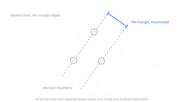
y_i (w^\top x_i + b) \geq 1 \quad \text{for every coin } i

The surfaces where the score is exactly $-1$ and $+1$ are the margin boundaries, dashed in the diagram. The gap between them is $2 / \lVert w \rVert$ , the length of the weight vector, so maximising the margin means minimising that length. Hence the objective $\tfrac{1}{2}\lVert w \rVert^2$ , convex, under straight-line constraints.

That's the hard margin, and it demands perfect separability. One 2-euro coin with a chunk missing, weighing 7.8 g, lands inside the other class's territory, and now no line satisfies all 240 constraints. The optimiser doesn't return something worse. It returns nothing.

Soft margin, and getting C the right way round

The repair: let points break the rule and charge for it. Each coin gets a slack $\xi_i$ , the amount it falls short by:

\tfrac{1}{2}\lVert w \rVert^2 + C \sum_i \xi_i

Everyone gets $C$ backwards, so read this twice. C is the price of a violation.

Large C makes violations expensive, so the optimiser contorts to satisfy every point and ends up with a narrow margin hugging the data — that damaged coin gets to move the boundary. Small C makes violations cheap, so it buys a wide margin and misclassifies some training points on purpose.

So C is a regularisation dial pointing the opposite way to most: turning it up regularises less.

Hinge loss, and why only nearby points matter

The slack sum has a name. For a coin with score $f(x)$ and label $y$ :

L = \max\big(0,\; 1 - y \, f(x)\big)

Read it as a rule about when the model stops caring. Get a coin right and clear of the margin and the loss is exactly zero. Not small. Zero. Inside the margin or on the wrong side, the cost grows in a straight line.

The log loss that logistic regression minimises never reaches zero, so a coin far out in correct territory still tugs on the boundary. Under hinge loss it contributes nothing.

That difference is the defining property. Only points inside or touching the margin have influence, so the solution rests on a handful of rows — the support vectors, three of them in the diagram. Delete every other coin and refit: identical answer. Compact, and exactly as trustworthy as those few rows. The output, note, is a signed distance to a hyperplane and not a probability.

Show Me the Code

C's direction, measured: plain subgradient steps on hinge loss plus an L2 penalty.

1import numpy as np2
3def fit(X: np.ndarray, y: np.ndarray, C: float, steps: int = 20000) -> np.ndarray:4    w = np.zeros(3)                                  # bias, then diameter and mass5    for t in range(1, steps + 1):6        inside = y * (X @ w) < 1.0                   # only points in or past the margin push back7        pull = C * (y[inside, None] * X[inside]).sum(axis=0) / len(y)8        w += (0.2 / t ** 0.5) * (pull - w * np.array([0.0, 1.0, 1.0]))9    return w10
11rng = np.random.default_rng(8)12y = np.where(np.arange(240) < 120, -1.0, 1.0)                    # -1 one euro, +1 two euro13diam = np.where(y < 0, 23.25, 25.75) + rng.normal(0.0, 0.45, 240)14mass = np.where(y < 0, 7.50, 8.50) + rng.normal(0.0, 0.22, 240)15X = np.column_stack([np.ones(240), diam - 24.5, mass - 8.0])     # centred so the bias starts near 016for C in (0.01, 1.0, 100.0):17    w = fit(X, y, C)18    print(f"C={C:6.2f}  margin width {2.0 / np.linalg.norm(w[1:]):5.2f}  "19          f"support vectors {int((y * (X @ w) <= 1.0 + 1e-3).sum()):3d}")20# -> C=  0.01  margin width 146.67  support vectors 24021# -> C=  1.00  margin width  3.01  support vectors 14822# -> C=100.00  margin width  1.31  support vectors  10

At C = 0.01 the margin is wider than the data, so every coin is a support vector and the model has given up. At C = 100 it collapses to 1.31 with ten coins defining the boundary. Up is tighter, every time.

Watch Out For

Tuning C in the direction you think you're tuning it

Someone decides the model is overfitting, reasons that C is a regularisation strength, and raises it from 1 to 100. Validation accuracy drops, so they raise it again, and it drops further.

The run labelled "heavily regularised" is the one hugging the data hardest. Check with a number instead of intuition: fit at two values of C and look at the margin width or the support-vector count. Few support vectors and a narrow margin means less regularisation. Log it in your sweep and you'll never have to remember the direction.

Reading the decision function as a probability

Push the decision function through a sigmoid and you get values between 0 and 1 that sort in the right order. They are not probabilities. The input was a signed distance in whatever units $\lVert w \rVert$ ended up with, so change C and every one of those numbers moves.

The symptom is quiet, because rankings stay fine: accuracy and AUC look healthy while any decision multiplying the number by a cost runs on fiction. Fit the mapping on held-out data, which is what probability calibration is for.

The Quick Version

Among all separating hyperplanes, this is the one furthest from the closest point on each side. Convex, so there's a single answer.
The margin width is $2 / \lVert w \rVert$ , so maximising it means minimising the weight vector's length.
Hard margin needs perfect separability; one outlier makes it infeasible. Soft margin adds slack.
Large C prices violations high: narrow margin, fits hard. Small C: wide margin, tolerates errors. Up means less regularisation.
Hinge loss hits exactly zero once a point is right and past the margin, so only nearby points shape the boundary. Those are the support vectors, and the model is only as trustworthy as they are.
The output is a signed distance, not a probability.