Core ML

The Kernel Trick

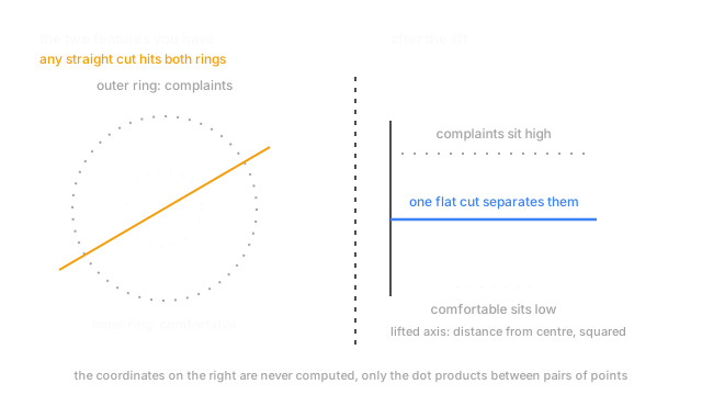
The algorithm never needs a point's coordinates in the huge new space, only dot products between pairs, so a kernel computes those and skips the projection.

Two rings that no straight line can separate become separable by a flat cut once one extra dimension is added, and the kernel gets the same answer without ever computing that dimension

Why Does This Exist?

An office building logs indoor temperature, relative humidity, and whether anyone filed a comfort complaint that hour. Thirty thousand hours of it, and facilities would like the room fixed before the email.

Plot it. Complaints come from too cold, too hot, too dry, too muggy — all four directions — so the comfortable hours sit in a blob ringed by complaints, as on the left of the diagram. No straight cut separates that, and the model isn't weak: a support vector machine draws one flat surface, and no flat surface has an inside and an outside.

The obvious repair works. Invent features by hand — temperature squared, humidity squared, temperature times humidity — and a flat cut in that space does the job, because a circle in the original features is a plane in the squared ones.

Then you try it on a real feature table. Every degree-2 combination of 1,000 features is 501,501 columns. Degree 3 is 167,668,501. The space you'd genuinely want, where the boundary curves however the data curves, is infinite-dimensional and cannot be built at all.

One thing to have straight: a dot product multiplies matching entries of two vectors and adds them up (details).

Think of It Like This

The courier's mileage chart

A courier plans a round trip between forty towns with no map and no coordinates. She has a chart of the road distance between every pair, and that's enough for everything she needs.

Now hand her a chart of driving times. It bends in ways no flat map reproduces — a mountain pass puts two nearby towns hours apart, a motorway makes two distant ones adjacent. She plans exactly as before, and her plan is correct in that stranger geometry, without anyone drawing it.

One catch. The chart must correspond to some real arrangement of towns, even one nobody can sketch. Invent numbers where A to B plus B to C is shorter than A to C and her plans are nonsense.

The kernel is the chart. The algorithm is the courier. No map gets drawn.

How It Actually Works

The algorithm only ever asks about pairs

Write out the trained form of a maximum-margin classifier and the feature vectors never appear on their own. They show up only inside dot products between pairs: two training points, or a training point with the one you're predicting. The algorithm never asks where a point sits in the expanded space — it asks for the dot product of two points there, one number per pair.

So if you can compute that number from the original features, the expansion is unnecessary. Not approximated. Never performed, with an identical answer. A function that does it is a kernel: $K(a, b) = \phi(a) \cdot \phi(b)$ , where $\phi$ is the projection you never evaluate.

The polynomial kernel, in one line

Take two feature vectors, compute their ordinary dot product, add 1, square it.

K(a, b) = (a \cdot b + 1)^2

That equals the dot product of all the degree-2 features of $a$ and $b$ : every squared term, every pairwise product, the original features, and a constant, with the coefficients that make the algebra line up. Expand the square by hand once and each group falls out.

Raise the exponent to 3 and you get every degree-3 interaction at the same price. The exponent dials curvature, and the cost never moves.

RBF, gamma, and which functions are allowed

The one you'll use most:

K(a, b) = \exp\big(-\gamma \lVert a - b \rVert^2\big)

Here $\lVert a - b \rVert^2$ is the squared distance between the two points and $\gamma$ is a positive number you pick. This one corresponds to an infinite-dimensional feature space — the case that could never be built — for one distance and one exponential.

Read $\gamma$ as reach. Small $\gamma$ keeps the value near 1 for points far apart, so each hour influences a wide region and the boundary is smooth. Large $\gamma$ collapses it to nearly zero for anything but immediate neighbours, so the boundary wraps tightly around individual rows. It pulls against C, so the two get tuned together.

Not every function you invent is a legal kernel. Mercer's condition is the requirement: the matrix of kernel values over any set of points must be positive semi-definite, so no combination of points has a negative squared length. Satisfy it and a feature space with these dot products provably exists. Break it and you're the courier with invented numbers.

What it cost. Every pair needs a kernel value, so training works with an $n \times n$ matrix. At 30,000 hours that's 900 million entries, 7.2 GB in double precision, growing with the square of your rows — which is why kernel methods went quiet as datasets grew.

Show Me the Code

An identity, not an approximation. Build the degree-2 space by hand, then square a dot product in the original 60 features.

1import itertools2import numpy as np3
4def lift(x: np.ndarray) -> np.ndarray:5    """Every degree-2 term, built explicitly, with the coefficients that make the algebra line up."""6    cross = [np.sqrt(2.0) * x[i] * x[j] for i, j in itertools.combinations(range(len(x)), 2)]7    return np.concatenate([x ** 2, np.array(cross), np.sqrt(2.0) * x, [1.0]])8
9def kernel(a: np.ndarray, b: np.ndarray) -> float:10    return float((a @ b + 1.0) ** 2)                 # same number, never leaving 60 columns11
12rng = np.random.default_rng(2)13a, b = rng.normal(size=60), rng.normal(size=60)14print(f"lifted:  {len(lift(a)):>9,} columns, dot product {lift(a) @ lift(b):.6f}")15print(f"kernel:  {len(a):>9,} columns, dot product {kernel(a, b):.6f}")16for d in (1_000, 10_000):17    print(f"at {d:,} features the lift would need {d * (d + 3) // 2 + 1:,} columns")18# -> lifted:      1,891 columns, dot product 76.88263119# -> kernel:         60 columns, dot product 76.88263120# -> at 1,000 features the lift would need 501,501 columns21# -> at 10,000 features the lift would need 50,015,001 columns

Same number, 1,891 columns against 60. At 10,000 features the honest expansion is 50 million columns per row; the kernel is still one dot product.

Watch Out For

Leaving gamma at a value tuned for other units

Gamma multiplies a squared distance, so it only means something relative to your feature scales. Switch temperature to Kelvin and the same gamma is a different reach entirely.

Too small and every kernel value sits near 1, so the model predicts one class everywhere. Too large and every value sits near 0 except a point with itself, so it memorises the training set. Standardise first, then search gamma on a log scale, jointly with C.

Reaching for a kernel on a large dataset

The quadratic matrix is not a footnote. At 30,000 rows you're at 7.2 GB; at 300,000 rows you're at 720 GB and the job doesn't run. Prediction is slow too, each new hour compared against every stored support vector.

So past a few tens of thousands of rows the kernel version is usually wrong even when it fits best. A linear model on a few hand-built interaction terms captures much of the same curvature at linear cost, and a boosted tree ensemble finds the interactions itself — which is why it took over the problems kernels used to own.

The Quick Version

No linear boundary separates a blob from the ring around it, and expanding features by hand explodes: 501,501 columns for degree 2 over 1,000 features.
Margin-based algorithms only ever use dot products between pairs. So a kernel computes that dot product from the original features and the projection never happens.
The polynomial kernel is one dot product, plus one, squared — equal to the dot product of every degree-2 feature.
The RBF kernel corresponds to an infinite-dimensional space, with gamma as reach. Standardise first, tune with C, and check your kernel satisfies Mercer's condition.
The bill is an $n \times n$ matrix: quadratic in rows, and the ceiling on the family.