Swin Transformer

Self-attention is computed inside small local windows that shift across consecutive layers to achieve linear computational complexity with image size.

Why Does This Exist?

The original Vision Transformer (ViT) calculates global self-attention across every patch in the image. If an image produces $N$ patch tokens, computing the pairwise attention matrix requires $\mathcal{O}(N^2)$ floating-point operations and memory. For a standard classification image of $224 \times 224$ pixels split into $16 \times 16$ patches, $N = 196$ , which is modest for modern accelerators.

However, dense computer vision tasks such as semantic segmentation and object detection require high-resolution inputs like $1024 \times 1024$ or $2048 \times 2048$ to delineate precise object boundaries. At $1024 \times 1024$ with $4 \times 4$ patches, the sequence length explodes to $N = 65,536$ . A single global attention matrix would require $(65,536)^2 \approx 4.29 \times 10^9$ elements per head, consuming over 17 gigabytes of GPU memory for one attention layer alone and triggering immediate out-of-memory crashes.

Furthermore, ViT produces single-scale feature maps at a constant downsampling factor ( $16\times$ ), making it incompatible with Feature Pyramid Networks (FPN) and UNet architectures that rely on multi-scale spatial representations.

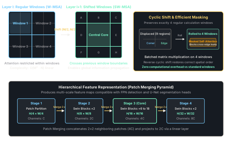
The Swin Transformer (Shifted Window Transformer) solves both problems. It restricts self-attention to small, fixed-size local windows of size $M \times M$ (typically $7 \times 7$ ), reducing computational complexity from quadratic $\mathcal{O}(N^2)$ to strictly linear $\mathcal{O}(M^2 N)$ . To allow information to cross window boundaries without reintroducing global computation, Swin shifts the window partitioning grid by half a window width in alternating layers. Optimization relies on gradient-descent across multi-scale backbones.

Think of It Like This

Staggered bricklaying across building floors

Imagine masons constructing a brick wall. On the first floor, bricks are laid side by side in neat pairs. If each pair of bricks is glued together internally (local window attention), the two bricks know each other perfectly, but no glue connects pair A to pair B. The wall would crack along the seams between pairs under slight pressure.

On the next floor, the masons do not stack bricks in identical columns. They shift every brick by half its width. The joint between the two bricks below now sits directly under the center of a solid brick above.

In the Swin Transformer, layer $\ell$ computes attention within static local windows (the pairs on the lower floor). Layer $\ell+1$ shifts the window boundaries by half a window. Patches that were separated at the borders in layer $\ell$ now find themselves inside the same window in layer $\ell+1$ . By alternating regular and shifted windows across successive layers, information flows seamlessly across the entire image canvas while keeping each mason's view strictly local.

How It Actually Works

Window and Shifted Window Multi-Head Attention

A feature map with $h \times w$ patches is partitioned into non-overlapping windows of size $M \times M$ patches. The computational complexities of standard global Multi-Head Self-Attention ( $\text{MSA}$ ) and Window-based Multi-Head Self-Attention ( $\text{W-MSA}$ ) for an image of $h \times w$ patches and hidden dimension $C$ are:

$\Omega(\text{MSA}) = 4hwC^2 + 2(hw)^2C$

$\Omega(\text{W-MSA}) = 4hwC^2 + 2M^2hwC$

When $M$ is fixed (commonly $M = 7$ ), $\Omega(\text{W-MSA})$ scales linearly with image area $hw$ , whereas $\Omega(\text{MSA})$ scales quadratically.

To enable cross-window communication, consecutive Swin Transformer blocks are deployed in pairs. The first block computes regular window attention ( $\text{W-MSA}$ ):

$\hat{z}^\ell = \text{W-MSA}(\text{LN}(z^{\ell-1})) + z^{\ell-1}$

$z^\ell = \text{MLP}(\text{LN}(\hat{z}^\ell)) + \hat{z}^\ell$

The second block computes Shifted Window attention ( $\text{SW-MSA}$ ) by translating the window partitioning grid by $(\lfloor \frac{M}{2} \rfloor, \lfloor \frac{M}{2} \rfloor)$ pixels from the top-left corner:

$\hat{z}^{\ell+1} = \text{SW-MSA}(\text{LN}(z^\ell)) + z^\ell$

$z^{\ell+1} = \text{MLP}(\text{LN}(\hat{z}^{\ell+1})) + \hat{z}^{\ell+1}$

Shifting the window grid creates up to 9 smaller sub-windows along the boundary edges. A naive approach would pad these sub-windows to size $M \times M$ , substantially increasing computation. Instead, Swin uses a cyclic shift: the boundary slices on the top and left are rolled to the bottom and right edges of the feature map, forming exactly $\lceil h/M \rceil \times \lceil w/M \rceil$ regular $M \times M$ windows.

Because cyclic rolling groups non-adjacent spatial regions together into the same window, a specialized attention mask is added during the dot-product computation:

$\text{Attention}(Q, K, V) = \text{softmax}\left(\frac{Q K^T}{\sqrt{d}} + B + \text{Mask}\right) V$

where $B$ is a learnable relative position bias matrix, and $\text{Mask}$ contains zeros for positions originating from the same spatial area and $-100$ (effectively $-\infty$ ) for mismatched regions, completely blocking spurious cross-boundary attention. After self-attention, a reverse cyclic shift restores the feature map to its original spatial layout.

Hierarchical Representation via Patch Merging

As the network goes deeper, resolution must decrease while channel capacity increases, matching standard vision pyramids. Swin achieves this through Patch Merging:

Groups of $2 \times 2$ neighboring patches are concatenated along the channel dimension, transforming a spatial patch tensor of shape $\frac{H}{2^k} \times \frac{W}{2^k} \times C$ into $\frac{H}{2^{k+1}} \times \frac{W}{2^{k+1}} \times 4C$ .
A linear projection layer maps the $4C$ channels to $2C$ .
The spatial resolution is halved while channel capacity doubles, creating feature maps at $\frac{H}{4}, \frac{H}{8}, \frac{H}{16},$ and $\frac{H}{32}$ scale.

Worked Example

Compare computational FLOPs on an input feature map of size $56 \times 56$ patches with window size $M = 7$ , channel dimension $C = 96$ , and total patch count $N = 56 \times 56 = 3,136$ :

Global Attention (ViT style):
- Self-attention matrix: $N \times N = 3,136 \times 3,136 = 9,834,496$ attention scores.
- Matrix multiplication FLOPs: $2 \times N^2 \times C = 2 \times (3,136)^2 \times 96 \approx 1,888,223,232$ FLOPs ( $\approx 1.89$ GFLOPs).
Swin Local Window Attention:
- Number of windows: $(56 / 7) \times (56 / 7) = 8 \times 8 = 64$ windows.
- Number of patches per window: $M^2 = 7 \times 7 = 49$ patches.
- Attention scores per window: $49 \times 49 = 2,401$ .
- Total attention scores across all 64 windows: $64 \times 2,401 = 153,664$ .
- Matrix multiplication FLOPs: $2 \times M^2 \times N \times C = 2 \times 49 \times 3,136 \times 96 \approx 29,503,488$ FLOPs ( $\approx 0.0295$ GFLOPs).

The local window mechanism achieves a 64-fold reduction in attention matrix computation while shifted windows guarantee cross-window receptive field propagation.

Code

1import torch2import torch.nn as nn3
4def window_partition(x: torch.Tensor, window_size: int) -> torch.Tensor:5    """Partitions a feature map into non-overlapping local windows.6    Args:7        x: Tensor of shape (B, H, W, C)8        window_size: Window dimension M9    Returns:10        windows: Tensor of shape (num_windows * B, window_size, window_size, C)11    """12    b, h, w, c = x.shape13    x = x.view(b, h // window_size, window_size, w // window_size, window_size, c)14    # Permute to (B, H/M, W/M, M, M, C) and flatten window batch15    windows = x.permute(0, 1, 3, 2, 4, 5).contiguous().view(-1, window_size, window_size, c)16    return windows17
18def window_reverse(windows: torch.Tensor, window_size: int, h: int, w: int) -> torch.Tensor:19    """Reverses window partition back to standard feature map layout."""20    b = int(windows.shape[0] / (h * w / window_size / window_size))21    x = windows.view(b, h // window_size, w // window_size, window_size, window_size, -1)22    x = x.permute(0, 1, 3, 2, 4, 5).contiguous().view(b, h, w, -1)23    return x24
25# Verify partition and reverse cyclic shift26batch_size, height, width, channels = 2, 14, 14, 9627window_size = 728feature_map = torch.randn(batch_size, height, width, channels)29
30# Partition into 4 windows per image -> total 8 windows31windows = window_partition(feature_map, window_size=window_size)32print("Windows shape:", windows.shape)33# -> Windows shape: torch.Size([8, 7, 7, 96])34
35# Reverse back to original spatial layout36reconstructed = window_reverse(windows, window_size=window_size, h=height, w=width)37print("Reconstruction matches input:", torch.allclose(feature_map, reconstructed))38# -> Reconstruction matches input: True39
40# Cyclic shift translation demonstration (shift_size = M // 2 = 3)41shift_size = window_size // 242shifted_x = torch.roll(feature_map, shifts=(-shift_size, -shift_size), dims=(1, 2))43print("Shifted tensor shape:", shifted_x.shape)44# -> Shifted tensor shape: torch.Size([2, 14, 14, 96])

Watch Out For

Information leakage in cyclic shifts without relative attention masking

When implementing Shifted Window Attention with cyclic shifts, boundary slices are rolled around the tensor to maintain a uniform rectangular grid. Consequently, a single $M \times M$ window in the bottom-right corner contains patches originating from four completely disconnected quadrants of the original image.

If self-attention is computed without an attention mask, tokens from the top-left corner attend directly to tokens from the bottom-right corner purely because they were rolled into the same computational buffer. This introduces artificial spatial shortcuts that corrupt position encoding and degrade segmentation boundaries. You must construct an attention mask containing large negative values (e.g. $-100.0$ ) between sub-regions that do not share true spatial proximity, ensuring the softmax sets their attention weight strictly to zero.

The Quick Version

Swin Transformer limits self-attention to non-overlapping local windows ( $M \times M$ ), reducing computational complexity from $\mathcal{O}(N^2)$ to strictly linear $\mathcal{O}(M^2 N)$ .
Alternating layers shift the window boundaries by half a window width, connecting neighboring regions and expanding the receptive field across the entire canvas.
Cyclic shifts and attention masking compute shifted-window attention with zero padding overhead, while Patch Merging builds a hierarchical multi-scale feature pyramid.