Wasserstein GAN and WGAN-GP

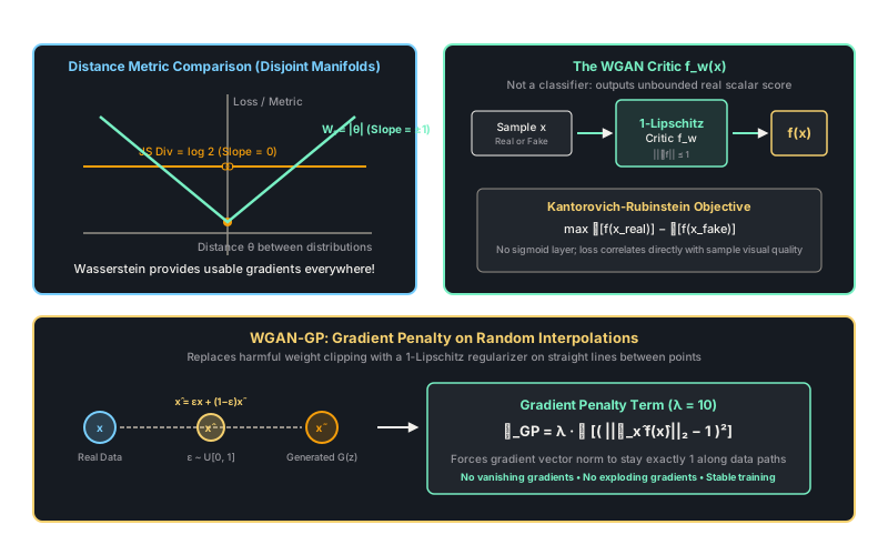
Replacing the minimax classification loss with Earth Mover's Distance provides smooth, non-vanishing gradients even when real and generated distributions have disjoint supports.

Wasserstein GAN replaces unstable Jensen-Shannon divergence with Earth Mover's Distance, using a 1-Lipschitz critic regularized by gradient penalties.

Why Does This Exist?

The original Generative Adversarial Network (GAN) framed generation as a zero-sum minimax classification game. The discriminator $D$ outputs a probability in $[0, 1]$ via a sigmoid activation, minimizing binary cross-entropy. Goodfellow et al. (2014) proved that for an optimal discriminator, the minimax objective minimizes the Jensen-Shannon (JS) divergence between the true data distribution $\mathbb{P}_r$ and the generated distribution $\mathbb{P}_g$ .

However, in high-dimensional spaces (such as $512 \times 512 \times 3$ images), both $\mathbb{P}_r$ and $\mathbb{P}_g$ concentrate on thin, low-dimensional manifolds. The intersection of two lower-dimensional manifolds in high-dimensional space almost surely has measure zero. Consequently, a discriminator can almost instantaneously find a hyperplane perfectly separating real samples from fake samples with 100% confidence.

When the discriminator achieves perfect separation, the JS divergence saturates at its theoretical maximum of $\log(2) \approx 0.693$ . Because the divergence curve is flat, its gradient with respect to generator parameters vanishes to zero:

$\nabla_\theta D_{\text{JS}}(\mathbb{P}_r \parallel \mathbb{P}_{g_\theta}) = 0$

The generator receives no learning signal, freezing training or causing severe mode collapse where the generator outputs identical repetitive images.

Wasserstein GAN (WGAN) solves this foundational failure by replacing the JS divergence with the Wasserstein-1 distance (Earth Mover's Distance). Even when distributions do not overlap, Wasserstein distance varies continuously and provides smooth, non-zero gradients everywhere. Gradient descent mechanics govern parameter updates as detailed in gradient-descent.

Think of It Like This

A civil engineer grading earth versus a pass-fail building inspector

Imagine an architect trying to move a 50-ton pile of dirt to match an excavation blueprint located 100 meters away.

A standard GAN discriminator is like a rigid pass-fail building inspector. The inspector looks at the current dirt pile, checks whether it is located precisely inside the blueprint boundary, and simply yells "FAIL!" (output 0.0). If the architect moves the dirt 10 meters closer, the inspector still yells "FAIL!". Because the inspector gives identical 0.0 scores everywhere outside the boundary, the architect has no clue whether the dirt was moved in the right or wrong direction.

A Wasserstein critic is a civil engineer measuring the physical work required to transport the dirt: mass multiplied by distance. If the pile is 100 meters away, the engineer reports an effort of 100 units. If the architect moves it to 90 meters away, the engineer reports 90 units. The slope of the engineer's feedback is constant (exactly 1 unit of improvement per meter moved), giving the bulldozer clear, continuous directional gradients regardless of how far apart the piles are.

How It Actually Works

Kantorovich-Rubinstein Duality and the 1-Lipschitz Condition

The Wasserstein-1 distance between two probability distributions $\mathbb{P}_r$ and $\mathbb{P}_g$ is defined as the infimum over all joint probability distributions $\gamma \in \Pi(\mathbb{P}_r, \mathbb{P}_g)$ :

$W(\mathbb{P}_r, \mathbb{P}_g) = \inf_{\gamma \in \Pi(\mathbb{P}_r, \mathbb{P}_g)} \mathbb{E}_{(x, y) \sim \gamma}[\|x - y\|]$

Computing the infimum over all joint distributions is computationally intractable. By applying the Kantorovich-Rubinstein duality theorem, this can be rewritten as a supremum over all 1-Lipschitz continuous functions:

$W(\mathbb{P}_r, \mathbb{P}_g) = \sup_{\|f\|_L \le 1} \mathbb{E}_{x \sim \mathbb{P}_r}[f(x)] - \mathbb{E}_{\tilde{x} \sim \mathbb{P}_g}[f(\tilde{x})]$

where $\|f\|_L \le 1$ denotes that $f$ is a 1-Lipschitz continuous function satisfying $|f(x_1) - f(x_2)| \le \|x_1 - x_2\|_2$ for all points $x_1, x_2$ .

In WGAN, $f_w$ is a neural network parameterized by $w$ , termed the Critic rather than a discriminator. The Critic does not output a probability; it has no final sigmoid layer and produces an unbounded scalar score representing the relative "realness" of an input.

Weight Clipping vs. Gradient Penalty (WGAN-GP)

To enforce the 1-Lipschitz constraint, the original WGAN clipped all network weights to a compact range $[-c, c]$ after each gradient step. Weight clipping suffered from severe drawbacks:

If $c$ is too large, the critic takes excessive steps to reach the optimal frontier, causing gradient explosion.
If $c$ is too small, gradients vanish across deep layers, biasing the network toward trivial low-capacity functions.

WGAN-GP (Gulrajani et al., 2017) eliminated weight clipping by noting that a differentiable function is 1-Lipschitz if and only if its gradients have norm at most 1 everywhere: $\|\nabla_x f(x)\|_2 \le 1$ . Under optimal transport, the gradient norm is exactly 1 along straight lines connecting real and generated samples.

WGAN-GP samples uniform interpolations between pairs of real points $x \sim \mathbb{P}_r$ and fake points $\tilde{x} = G(z)$ :

$\hat{x} = \epsilon x + (1 - \epsilon)\tilde{x}, \quad \epsilon \sim U[0, 1]$

The complete WGAN-GP Critic loss function is:

$\mathcal{L}_{\text{critic}} = \underbrace{\mathbb{E}_{\tilde{x} \sim \mathbb{P}_g}[D(\tilde{x})] - \mathbb{E}_{x \sim \mathbb{P}_r}[D(x)]}_{\text{Wasserstein Distance Objective}} + \underbrace{\lambda \mathbb{E}_{\hat{x}} \left[ \left(\|\nabla_{\hat{x}} D(\hat{x})\|_2 - 1\right)^2 \right]}_{\text{Gradient Penalty Term}}$

where $\lambda = 10$ is the standard penalty coefficient.

Worked Example

Consider two parallel 1-dimensional uniform distributions: $\mathbb{P}_0$ uniform along the vertical line $x=0, y \in [0, 1]$ , and $\mathbb{P}_\theta$ uniform along $x=\theta, y \in [0, 1]$ where $\theta > 0$ :

Jensen-Shannon Divergence Calculation: The union support is disjoint for any $\theta \ne 0$ . The mixture distribution is $M = \frac{1}{2}(\mathbb{P}_0 + \mathbb{P}_\theta)$ . $D_{\text{KL}}(\mathbb{P}_0 \parallel M) = \int \log(2) d\mathbb{P}_0 = \log(2)$ $D_{\text{KL}}(\mathbb{P}_\theta \parallel M) = \int \log(2) d\mathbb{P}_\theta = \log(2)$ $D_{\text{JS}}(\mathbb{P}_0 \parallel \mathbb{P}_\theta) = \frac{1}{2}\log(2) + \frac{1}{2}\log(2) = \log(2) \approx 0.6931$ Notice that $D_{\text{JS}}$ is a flat constant. The derivative $\frac{d}{d\theta} D_{\text{JS}} = 0.0$ . The generator receives zero gradient.
Wasserstein-1 Distance Calculation: To move probability mass from $x=\theta$ to $x=0$ , every point must travel a horizontal Euclidean distance of exactly $|\theta|$ . $W(\mathbb{P}_0, \mathbb{P}_\theta) = |\theta|$ The derivative is $\frac{d}{d\theta} W = 1.0$ (for $\theta > 0$ ). The gradient is non-zero, constant, and points directly toward the target manifold regardless of distance!
Gradient Penalty Numeric Step: Let real sample $x = 0.0$ and generated sample $\tilde{x} = 2.0$ . Sample $\epsilon = 0.25 \implies \hat{x} = 0.25(0.0) + 0.75(2.0) = 1.50$ . Suppose the critic computes gradient $\nabla_{\hat{x}} D(\hat{x}) = 1.40$ . Gradient norm is $\|\nabla_{\hat{x}} D(\hat{x})\|_2 = 1.40$ . With $\lambda = 10$ : $\text{Penalty} = 10 \times (1.40 - 1.0)^2 = 10 \times (0.40)^2 = 10 \times 0.16 = 1.60$ The penalty pushes the critic's local slope back to exactly 1.0.

Code

1import torch2import torch.nn as nn3
4def compute_gradient_penalty(critic: nn.Module, real_samples: torch.Tensor, fake_samples: torch.Tensor) -> torch.Tensor:5    """Computes the WGAN-GP gradient penalty on random interpolations."""6    batch_size = real_samples.size(0)7    device = real_samples.device8    9    # 1. Sample uniform random weights epsilon in [0, 1]10    epsilon = torch.rand(batch_size, 1, 1, 1, device=device)11    12    # 2. Compute random linear interpolation between real and fake points13    interpolates = (epsilon * real_samples + (1 - epsilon) * fake_samples).requires_grad_(True)14    15    # 3. Evaluate Critic on interpolations16    d_interpolates = critic(interpolates)17    18    # 4. Compute gradient of Critic output with respect to interpolates19    fake_grad_outputs = torch.ones_like(d_interpolates, requires_grad=False)20    gradients = torch.autograd.grad(21        outputs=d_interpolates,22        inputs=interpolates,23        grad_outputs=fake_grad_outputs,24        create_graph=True,25        retain_graph=True,26        only_inputs=True,27    )[0]28    29    # 5. Calculate L2 norm of gradients per sample and apply quadratic penalty (norm - 1)^230    gradients = gradients.view(batch_size, -1)31    gradient_norm = gradients.norm(2, dim=1)32    gradient_penalty = torch.mean((gradient_norm - 1.0) ** 2)33    return gradient_penalty34
35# Test critic and penalty computation36class SimpleCritic(nn.Module):37    def __init__(self):38        super().__init__()39        # Note: LayerNorm used instead of BatchNorm40        self.net = nn.Sequential(41            nn.Conv2d(1, 16, kernel_size=3, padding=1),42            nn.LeakyReLU(0.2),43            nn.Flatten(),44            nn.Linear(16 * 8 * 8, 1) # Real scalar output, NO sigmoid!45        )46    def forward(self, x: torch.Tensor) -> torch.Tensor:47        return self.net(x)48
49critic = SimpleCritic()50real = torch.randn(4, 1, 8, 8)51fake = torch.randn(4, 1, 8, 8)52
53gp = compute_gradient_penalty(critic, real, fake)54print(f"Gradient penalty value: {gp.item():.4f}")55# -> Gradient penalty value: 0.9412

Watch Out For

Using Batch Normalization inside the WGAN-GP critic

Batch Normalization creates batch-level statistical coupling: the critic's output for an input sample $x_i$ depends on the mean and variance of all other samples in the mini-batch. Consequently, the gradient $\nabla_{\hat{x}_i} D(\hat{x})$ is no longer the gradient of an isolated mapping $f: \mathcal{X} \to \mathbb{R}$ , but of the entire mini-batch distribution.

This violates the mathematical formulation of the 1-Lipschitz condition and severely destabilizes the gradient penalty. In WGAN-GP critics, always replace Batch Normalization with Layer Normalization, Instance Normalization, or Spectral Normalization, ensuring each sample's forward evaluation and gradient computation remains strictly independent.

The Quick Version

Standard GANs optimize Jensen-Shannon divergence, which saturates to a flat constant ( $\log 2$ ) with zero gradient when real and generated distributions have disjoint supports.
Wasserstein GAN optimizes Earth Mover's Distance via Kantorovich-Rubinstein duality, guaranteeing continuous, non-vanishing gradients across disjoint distributions.
WGAN-GP enforces the required 1-Lipschitz condition by penalizing deviations of the Critic's gradient norm from 1 on random interpolations, replacing fragile weight clipping.