Data Concepts

Feature Construction

This is where you add what the table doesn't already know. A ratio, a lag, a count in a window — and every one of them computed as of the prediction time.

A raw order table becomes three constructed columns, and the vertical line at prediction time is what decides which events are allowed to contribute

Why Does This Exist?

Scaling a column has roughly one right answer. Encoding one has about four, and cardinality picks. Construction has no answer until somebody knows something about the problem, which is why it holds the most headroom and the least automation.

A model combines your columns only in the ways its own family permits. A linear model adds them up; a tree cuts them one at a time, along axes. Neither divides two columns by each other, and neither knows that 03:00 on a Tuesday means something different from 13:00 on a Saturday. That knowledge lives in your head, or a domain expert's, or a table nobody joined. Construction writes it into the feature matrix as a column — the only step that adds information rather than rearranging it.

Think of It Like This

Two price tags and a tape measure

Two flats, both listed at £420,000. The sheet in your hand has the price and the floor area, so anything reading it sees two numbers and no argument.

The first flat is 55 square metres: £7,636 per square metre. The second is 92, which works out at £4,565. Same headline price, and one is nearly twice the deal.

Nobody printed £/m² on that sheet. You worked it out, because a price means nothing until you divide it by what you're getting. Then you wrote it down as a number, before anyone reasoned with it. That's the discipline.

How It Actually Works

The moves worth knowing

Nearly every good tabular feature is one of about eight shapes.

Ratios and rates. Price per square metre, clicks per impression, debt-to-income. Dividing by size is the highest-yield move on tabular data.
Differences and deltas. Promised delivery date minus actual, current reading minus the rolling mean.
Date and time parts. Hour, day of week, is-weekend, days since signup, days until the next holiday. A raw timestamp only ever grows, so any split on it means "before or after this date".
Aggregations over a group. Orders per customer, mean basket value, max session length, distinct devices.
Lags and windows. Yesterday's value, the 7-day rolling mean, an expanding count since signup. A lag feature is how a model reaches the past.
Counts in a trailing window. Failed payments in the last 30 days, logins in the last 24 hours. Heavy hitters in fraud and churn.
Flags for a business rule. is_first_order, exceeds_credit_limit. Often what a domain expert would name first.
Interaction terms. The product of two columns, is_premium × discount_pct — an interaction feature is you doing the multiplication a linear model's form forbids.

A ratio costs you one line and costs a tree a staircase of dozens of splits that only approximates it.

As of when

One sentence separates a feature from a bug. Every aggregate and every window has to be computed as of the moment you'd actually have to predict.

Not as of today, and not as of whenever the export ran. As of the prediction timestamp for that row — so a customer's mean_order_value differs between a January row and a June row. If it doesn't, you've built something that cannot exist in production.

Warehouses make the wrong version easier to write: GROUP BY customer_id over the whole table, joined onto a January row, looks tidy. The right version recomputes per row against only the events before that row's timestamp, which is what an as-of join does — see SQL for feature extraction. The split obeys the same clock, so a time dimension means a temporal cut: train, validation and test splits.

Worked example

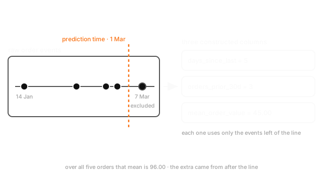
One customer, five orders, and a churn model scoring them on 1 March 2026: 14 Jan £40, 6 Feb £55, 19 Feb £25, 24 Feb £60, 7 Mar £300. That last order sits on the wrong side of the line. It's in the table you build features from today, and it did not exist on 1 March.

days_since_last_order is 1 March minus 24 February, so 5. orders_in_prior_30d counts back to 30 January, catching 6 Feb, 19 Feb and 24 Feb, so 3. mean_order_value is $(40 + 55 + 25 + 60) / 4 = 45.00$ .

Build that last one over every row instead: $(40 + 55 + 25 + 60 + 300) / 5 = 96.00$ . Same column name, more than double the value, and the extra came from an order placed six days after the prediction. Nothing is null, nothing errors, and your validation score goes up.

Show Me the Code

1import numpy as np2
3stamps = np.array(["2026-01-14", "2026-02-06", "2026-02-19", "2026-02-24", "2026-03-07"],4                  dtype="datetime64[D]")5amounts = np.array([40.0, 55.0, 25.0, 60.0, 300.0])   # the last order lands AFTER the cut6
7
8def features_as_of(t: np.ndarray, amt: np.ndarray, cut: np.datetime64) -> dict[str, float]:9    known = t < cut                                   # the whole discipline lives on this line10    days = (cut - t[known]) / np.timedelta64(1, "D")11    return {12        "days_since_last": float(days.min()),13        "orders_prior_30d": float((days <= 30).sum()),14        "mean_order_value": float(amt[known].mean()),15    }16
17feats = features_as_of(stamps, amounts, np.datetime64("2026-03-01"))18print(feats)                  # -> {'days_since_last': 5.0, 'orders_prior_30d': 3.0, 'mean_order_value': 45.0}19print(float(amounts.mean()))  # -> 96.0   same column over all time, and that is the leak

Drop known and the mean goes to 96.0, the count picks up a future order, and days_since_last turns into −6 — the only visible symptom.

Watch Out For

An aggregate that quietly averages the future

mean_order_value computed with one GROUP BY over the whole history, then joined onto every training row. No null, no error, no column name that sounds suspicious.

A row dated 12 January carries a mean built partly from orders in March and November. The model learns that customers with a high lifetime mean don't churn — true and useless, because the high mean is partly caused by not churning. In production the column is computed from data that exists, the distribution moves, and your best feature stops working.

The tell: a feature that ranks first on importance, costs nothing when removed under a random split, and costs a lot under a time-ordered backtest. Believe the backtest, then fix it structurally — every aggregate as an as-of value keyed on the row's timestamp, validated on a temporal split. See data leakage.

Generating a thousand ratios and shipping all of them

Forty numeric columns give 780 pairs, so 2,340 candidates once you divide, multiply and subtract each one. You keep the top 200 by importance, validation lands a shade above baseline, and you ship.

Here's what went wrong. With 2,340 candidates and a few thousand rows, some pure-noise columns score well by luck — that's what selection does once the pool is big enough. They survive, and the model gets worse while its feature list looks richer.

Generating candidates is fine. Selecting from them with the data you report on is not. Nest selection inside cross-validation folds, keep a final untouched split, and expect most to die. Automated feature engineering goes further.

The Quick Version

Construction is the only step that adds information. Encoding, scaling and selection rearrange what's there.
Eight shapes cover most of it: ratios, differences, date parts, group aggregates, lags and windows, trailing counts, rule flags, interactions.
Dividing by size is the highest-yield move on tabular data. A raw timestamp is nearly useless; its parts are strong.
Neither trees nor linear models divide one column by another.
Every aggregate and every window is computed as of the row's prediction time.
The same aggregate over all history is a leak with no null in it: 45.00 becomes 96.00, silently.
Generating thousands of candidates is fine. Selecting from them with the data you report on is not.