Data Concepts

Graph and Network Data

Here the data is the relationships, so the one-row-per-thing assumption breaks. How you store the edges decides what you can compute and how you must split.

One edge between two nodes shows up three ways — a pair in an edge list, a cell in an adjacency matrix, and an entry in a neighbour list — and the choice decides what you can compute at scale

Why Does This Exist?

A fraud team has a table of accounts and a table of transfers. Every model they build tops out around the same accuracy, because the accounts table describes accounts and the fraud is in the pattern of transfers: three accounts moving money in a ring, a new device shared by forty users, a merchant one hop from six known mules.

None of that is a column. It's a shape, spread across rows, and it only exists once you treat the transfers as edges.

That breaks the assumption every other page in this band rests on. There, a row is one thing and rows are independent. Here the data is the relationships between things, so the interesting unit spans many rows and nothing is independent of its neighbours.

This page is about storing, featurising and splitting graphs. The mathematics of graphs — paths, connectivity, spectra — is graph fundamentals.

Think of It Like This

A phone book, or a pile of call records

Two ways to hand someone a social network.

The first is a giant grid: everyone down the side, everyone across the top, a tick where two people know each other. Checking whether Ana knows Ben takes one glance at one cell. The problem is size — a thousand people means a million cells, and a million people means a trillion, nearly all of them empty, because nobody knows a million people.

The second is a stack of cards, one per friendship. Ten thousand friendships, ten thousand cards, and the pile grows with the friendships rather than with the square of the population. Now "does Ana know Ben" means going through the pile.

So you file the cards by name. One drawer per person, holding only their friendships. Small, and Ana's drawer answers instantly.

That third thing is how every real graph is stored.

How It Actually Works

Three storage forms, and the arithmetic that picks one

An adjacency matrix is $n \times n$ with a one where an edge exists. Constant-time edge lookup, and a memory cost in the square of your node count: a million nodes is $10^{12}$ cells, which is a terabyte even at one byte each. Dense storage is off the table above a few tens of thousands of nodes.

An edge list is two columns, one row per edge, so memory grows with edges rather than with nodes squared. Ten million edges is about 160MB at two 64-bit integers each. Compact, and answering "who are Ana's neighbours" means scanning the whole thing.

CSR-style adjacency sorts the edge list by source and stores an index of where each node's neighbours begin — the same sparse matrix layout the rest of the band uses. Linear memory, O(1) access to a node's neighbour block. This is what graph libraries actually use.

What carries the features

Nodes carry features (account age, device count). Edges carry features and weights (amount, timestamp, direction). The graph itself can carry attributes. And direction matters: a follow is one-way, a transfer is one-way, a friendship isn't, and an undirected edge is stored as two entries.

A heterogeneous graph has several node types and several edge types — accounts, devices, merchants; transfers, logins, ownership. One adjacency matrix can't express that, so you keep one per edge type.

Featurising, cheapest first

Structural features per node: degree, weighted degree, clustering coefficient, triangle count, PageRank, betweenness. Compute them, put them in an ordinary tabular model beside your existing columns, and you have captured most of the available lift for a fraction of the work. Start here.

Random-walk embeddings next. Generate random walks from each node, treat each walk as a sentence of node ids, and train a word-embedding model on them — that's node2vec and DeepWalk, and it works because "appears in similar walks" is a good proxy for "sits in a similar part of the graph". The output is a vector per node, so everything on vector embeddings applies.

Message passing learns node representations by repeatedly aggregating from neighbours. That's a modelling subject rather than a data one, so it belongs elsewhere.

Splitting a graph is where it goes wrong

Transductive: the whole graph structure is visible during training and you hide only some labels. Reasonable for a fixed network you're labelling once.

Inductive: whole nodes or subgraphs are held out, structure included, so the model must handle a node it has never seen. This is what production almost always means, because tomorrow's accounts don't exist yet.

Those give very different numbers, and a transductive experiment reported as an inductive capability is a common overclaim.

Link prediction has its own trap. You're predicting whether an edge exists, so every edge you're evaluating on must be removed from the structure the model reads. Leave it in and the answer is one of the inputs.

And a graph with timestamps on its edges is a time series too, so the split has to be temporal as well as structural.

Worked example

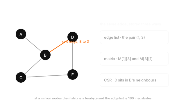
Five nodes, A to E, with edges A–B, B–C, B–D, D–E and C–E.

The edge list is five pairs. The adjacency matrix is $5 \times 5 = 25$ cells holding ten ones, because each undirected edge appears twice — so row sums give degrees directly: A has 1, B has 3, C has 2, D has 2, E has 2. Those sum to 10, which is twice the edge count, as they must.

Density is $10/25 = 40\%$ , which is why a matrix is fine at five nodes.

Now scale it. A million nodes with ten million edges: the matrix is $10^{12}$ cells, so 1TB at one byte each. The edge list is $10^7 \times 2 \times 8$ bytes, so 160MB. Same graph, a factor of 6,000 apart, and the matrix is 99.999% zeros.

Show Me the Code

1import numpy as np2
3edges: list[tuple[int, int]] = [(0, 1), (1, 2), (1, 3), (3, 4), (2, 4)]  # A-B B-C B-D D-E C-E4n: int = 55A: np.ndarray = np.zeros((n, n), dtype=np.int8)6for u, v in edges:7    A[u, v] = A[v, u] = 1                      # undirected, so every edge is stored twice8
9def dense_bytes(nodes: int) -> int:10    return nodes * nodes                        # one byte per cell, the cheapest dense form11
12def edge_list_bytes(edge_count: int) -> int:13    return edge_count * 2 * 8                   # two int64 endpoints per edge14
15print(A.sum(axis=1).tolist())                   # -> [1, 3, 2, 2, 2]   degrees16print(int(A.sum()), len(edges) * 2)             # -> 10 10             twice the edges17print(dense_bytes(1_000_000) / 1e12)            # -> 1.0    terabytes for a million nodes18print(edge_list_bytes(10_000_000) / 1e6)        # -> 160.0  megabytes for the same graph

Row sums giving degrees is the useful identity. The last two lines are why nobody builds the matrix.

Watch Out For

Predicting an edge the model can already see

You're scoring whether two accounts will transact. You build the graph, compute node embeddings, take the positive examples from existing edges, sample negatives, and get 0.99 AUC on the first run.

The embeddings were trained on a graph that contained those edges. Two nodes joined by an edge end up adjacent in embedding space because of that edge, so the feature encodes the answer. It's target leakage with a graph algorithm in between, and it's the single most common mistake in applied link prediction.

Remove the evaluation edges from the structure before computing anything — features, embeddings, walks, all of it — then rebuild. The score drops a long way and starts being real.

Two related versions. Structural features like common-neighbour count silently include the edge unless you drop it first. And negative sampling matters: sampling random non-edges makes the task far easier than sampling plausible ones, because most random pairs are trivially unrelated.

A dense matrix, or an inductive claim from a transductive test

np.zeros((n, n)) at 200,000 nodes asks for 40 billion cells and 320GB. The line looks harmless because it works perfectly at 500 nodes in a notebook, then the same code meets the real graph. Use an edge list or a CSR adjacency from the start, and never materialise the matrix to compute a degree.

The split half is quieter. Hold out labels while leaving the whole structure visible, report the number, and ship it as "the model handles new accounts". It doesn't: at training time every held-out node's neighbours, features and position were all available, and a new account has none of that.

Hold out whole nodes with their edges, and if edges carry timestamps, cut by time as well — temporal splitting applies here exactly as it does to a table.

The Quick Version

The data is the relationships, so the interesting unit spans rows and nothing is independent of its neighbours.
An adjacency matrix costs $n^2$ : a million nodes is a terabyte. An edge list costs $O(E)$ : the same graph is 160MB. CSR adjacency gives linear memory with O(1) neighbour access, and it's what real libraries use.
Nodes, edges and the graph can all carry features. Direction matters, and a heterogeneous graph needs one adjacency structure per edge type.
Start with structural features — degree, triangles, PageRank, clustering coefficient — in an ordinary tabular model. Most of the lift, very little of the work.
Random-walk embeddings turn walks into sentences and reuse word-embedding machinery, giving one vector per node.
Transductive means the structure is visible and labels are hidden. Inductive means whole nodes are held out, and that's what production means.
For link prediction, delete the evaluation edges from the structure before computing anything. Otherwise the answer is an input.
Edge timestamps make the graph a time series, so split by time too.