Math

Graph Fundamentals

Things and the connections between them — and the useful surprise that writing those connections in a grid turns the whole picture into a matrix you can do algebra on.

A graph and a matrix are the same object written two ways: put a one wherever an edge exists and the picture becomes an adjacency matrix that linear algebra can operate on

Why Does This Exist?

Three of the most important structures in machine learning are graphs, and they are usually taught without anyone saying so.

The autodiff tape is a graph. Your framework records every operation as a node and every data dependency as an edge, then walks that structure backwards to compute gradients. The chain rule says backpropagation is itself applied "over a computational graph" — this page is where that phrase gets a definition, and computational graphs is where it gets built.

A graph neural network's input is a graph. Molecules, social networks, road systems, knowledge bases. GNNs exist because the data has no grid to slide a convolution over.

Attention is a graph. Every token attending to every other token is a complete weighted directed graph, and the attention matrix is its adjacency matrix. Causal masking is the operation that turns it into a directed acyclic graph.

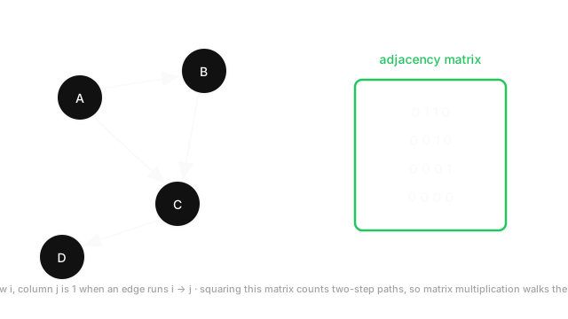
The payoff of this page is the bridge in the diagram: a graph written as a matrix means every tool from the linear algebra section applies to it. Matrix multiplication counts paths. Eigenvalues describe connectivity. That is not an analogy — it is the same arithmetic.

Think of It Like This

A city's one-way streets, written as a table

A city map shows junctions and the roads between them. Some roads are one-way. You can walk it visually — trace a route, spot a dead end, notice a loop.

Now write it as a table instead. One row and one column per junction, and a 1 in a cell when a road runs from that row's junction to that column's junction. Same city, no information lost, and the visual intuition is gone.

What you gain is arithmetic. Multiply that table by itself and each cell tells you how many two-road routes connect those junctions. Multiply again for three-road routes. You have replaced tracing paths by eye with matrix multiplication, and a computer can do the second thing on a graph with a billion junctions.

One asymmetry worth noticing: a two-way street puts a 1 in two cells, symmetric about the diagonal. A one-way street puts a 1 in one. So the matrix being symmetric tells you at a glance whether the city has any one-way roads at all.

How It Actually Works

A graph $G = (V, E)$ is a set of vertices (nodes) and a set of edges (pairs of vertices). That is the entire definition. The variations that matter:

Directed vs undirected. A directed edge goes one way; an undirected edge both. Friendship is undirected, "follows" is directed.
Weighted vs unweighted. An edge can carry a number — a distance, a cost, an attention score.
Cyclic vs acyclic. A cycle is a path returning to its start. A directed graph with none is a DAG, and DAGs are the important case for ML because they can be ordered.
Degree. How many edges touch a node. Directed graphs split this into in-degree and out-degree.

The adjacency matrix is the bridge

For a graph with $n$ nodes, the adjacency matrix $A$ is $n \times n$ with

A_{ij} = \begin{cases} 1 & \text{if an edge runs } i \to j \\ 0 & \text{otherwise} \end{cases}

In plain words: one row and column per node, marked where edges exist. For a weighted graph, store the weight instead of the 1.

Three facts do most of the work:

$A$ is symmetric exactly when the graph is undirected. So symmetry is a structural property you can test with one comparison.
Row sums give out-degree; column sums give in-degree. For an undirected graph they agree.
$(A^k)_{ij}$ counts the walks of length exactly $k$ from $i$ to $j$ . This is the result that makes the whole translation worthwhile, and it is just matrix multiplication: the sum over intermediate nodes of "can I get to $p$ " times "can I get from $p$ to $j$ " is precisely the definition of a matrix product.

That third fact is also, essentially, what a graph neural network layer does. One round of message passing aggregates each node's neighbours, and stacking $k$ layers lets information travel $k$ hops — the same reach as $A^k$ .

Topological order, and why DAGs matter

A DAG can be linearised: arrange its nodes so every edge points forward. That arrangement is a topological order, and it exists if and only if the graph has no cycles.

This is the property autodiff depends on. Run the operations in topological order and every input is ready before it is needed. Reverse that order for the backward pass and every gradient is available when required. No cycles means no chicken-and-egg, which is why frameworks build DAGs and why a cycle in your graph is a bug rather than a slow path.

Sparsity is the practical constraint

Most real graphs are sparse — a social network with a billion users does not have a billion friends per user. A dense adjacency matrix would need $n^2$ entries, which at $n = 10^6$ is $10^{12}$ numbers, or 4 TB in float32.

So real implementations store edge lists or compressed sparse formats, and the cost of an operation depends on the edge count $|E|$ rather than $n^2$ . This is why GNN libraries use scatter-gather primitives instead of dense matmuls, and why a dense attention matrix costing $O(n^2)$ in sequence length is the transformer's central scaling problem — attention is the rare case where the graph genuinely is complete.

Worked example

Take the four-node directed graph in the diagram: edges A→B, A→C, B→C, C→D. Ordering the nodes A, B, C, D:

A = \begin{bmatrix} 0 & 1 & 1 & 0 \\ 0 & 0 & 1 & 0 \\ 0 & 0 & 0 & 1 \\ 0 & 0 & 0 & 0 \end{bmatrix}

Row A has 1s in columns B and C, matching its two outgoing edges. Out-degrees are the row sums: A has 2, B has 1, C has 1, D has 0. In-degrees are the column sums: A has 0, B has 1, C has 2, D has 1.

The matrix is not symmetric, correctly reflecting a directed graph. And every 1 sits above the diagonal, which is the signature of a graph already written in topological order — A, B, C, D is a valid ordering, since every edge points to a later letter.

Now square it to count two-step walks:

A^2 = \begin{bmatrix} 0 & 0 & 1 & 1 \\ 0 & 0 & 0 & 1 \\ 0 & 0 & 0 & 0 \\ 0 & 0 & 0 & 0 \end{bmatrix}

Check one entry by hand. $(A^2)_{A,D} = 1$ , claiming exactly one two-step walk from A to D. Trace it: A→C→D. Correct, and A→B→C is the other two-step walk, showing up as $(A^2)_{A,C} = 1$ . Note $(A^2)_{A,B} = 0$ — there is a one-step route A→B but no two-step one, and $A^2$ counts walks of length exactly two.

Show Me the Code

1import numpy as np2
3# Nodes ordered A, B, C, D. Edges: A->B, A->C, B->C, C->D.4A = np.array([[0, 1, 1, 0],5              [0, 0, 1, 0],6              [0, 0, 0, 1],7              [0, 0, 0, 0]])                 # shape (4, 4)8
9print(A.sum(axis=1))                          # -> [2 1 1 0]  out-degree per node10print(A.sum(axis=0))                          # -> [0 1 2 1]  in-degree per node11print(np.array_equal(A, A.T))                 # -> False      so it is directed12
13print((A @ A)[0].tolist())                    # -> [0, 0, 1, 1]  2-step walks from A14print(np.trace(A @ A @ A))                    # -> 0   no 3-cycles, consistent with a DAG15
16# Upper-triangular means A, B, C, D is already a topological order.17print(np.allclose(A, np.triu(A, k=1)))        # -> True

Every number matches the hand calculation. The trace check is a genuinely useful trick: a nonzero trace of $A^k$ means a closed walk of length $k$ exists, so it detects cycles.

Watch Out For

Building a dense adjacency matrix for a real graph

The matrix view is the right way to think and usually the wrong way to store.

A graph with a million nodes has a dense adjacency matrix of $10^{12}$ entries — about 4 TB in float32. If the average node has 10 neighbours, the actual information is 10 million edges, which fits comfortably in memory. The dense form is a hundred thousand times larger than the data.

The failure mode is not a clean out-of-memory error, either. Code written against dense matrices works on the toy graph in the tutorial, works on the 10,000-node sample, and then either exhausts memory or slows to a crawl on the real dataset — after the architecture has been built around it. Refactoring dense matmuls into scatter-gather operations late is painful.

Use scipy.sparse or your GNN framework's edge-index format from the start, and reason about cost in terms of $|E|$ rather than $n^2$ . Reach for the dense matrix only when the graph genuinely is dense — which, for attention over a sequence, it is, and that is exactly why attention has a quadratic scaling problem.

Letting a cycle into a graph that must be acyclic

Anything that needs a topological order needs the graph to be a DAG, and a single cycle removes the ordering entirely — not degrading it, eliminating it.

In autodiff this appears as an in-place operation that overwrites a value the backward pass still needs, or a tensor reused in a way that makes a node its own ancestor. PyTorch raises on some of these and produces silently wrong gradients on others, which is worse. The classic symptom is a RuntimeError about a variable needed for gradient computation having been modified, and the classic cause is x += y where x = x + y was meant.

It also appears in data. A dependency graph with a cycle cannot be scheduled; a causal graph with a cycle is not a causal graph; an "is-a" hierarchy scraped from real data frequently contains loops that break any traversal assuming a tree.

The defence is to check rather than assume. np.trace(A @ A) nonzero means a 2-cycle, and any topological-sort routine fails loudly on a cyclic graph — which makes running one a cheap validity test rather than just a scheduling step.

The Quick Version

A graph is vertices plus edges. Directed or not, weighted or not, cyclic or not.
The adjacency matrix puts a 1 (or a weight) wherever an edge exists — same information, now open to linear algebra.
Symmetric adjacency matrix ⟺ undirected graph. Row sums are out-degree, column sums in-degree.
$(A^k)_{ij}$ counts walks of length exactly $k$ , so matrix multiplication traverses the graph. This is essentially what stacked GNN layers do.
A DAG has no cycles, so its nodes can be put in topological order. That is what makes autodiff possible.
Upper-triangular adjacency means the node ordering is already topological.
Real graphs are sparse: store edges, and reason about cost in $|E|$ , not $n^2$ .
Attention is the rare dense case — a complete weighted graph, which is why it costs $O(n^2)$ .