Data Concepts

Time-Series and Temporal Data

Ordering is information, and every default in your toolkit assumes it isn't. Shuffle these rows and you have destroyed the exact thing you were modelling.

An expanding-window backtest trains only on rows earlier than the block it validates, and the gap between the two is what stops a label that spans time from crossing the cut

Why Does This Exist?

A demand forecast validates at 0.91 and loses money in its first week.

The line that did it is train_test_split(X, y, random_state=42). March rows went into training, February rows into validation, so the model was asked to fill in a gap between two things it had already seen. Interpolation is much easier than forecasting, and nothing in the code says which one you measured.

Every other page in this band treats rows as interchangeable: shuffle them, and the dataset is the same dataset. Here it isn't. The order is part of the data, and most of the signal lives in how consecutive values relate rather than in the values themselves.

The vocabulary, in one paragraph

A time series is values indexed by time. Regular sampling means one row per fixed interval, so a daily sales table is regular. Irregular means rows arrive whenever something happened, so a click log is irregular and most joins on it are wrong by default. Event time is when the thing happened; processing time is when your system saw it. Those two agree until something arrives late, and then they disagree permanently for that row.

Think of It Like This

A film cut into frames and shuffled

Take a film apart into single frames and shuffle the pile. Every frame is intact. You can still describe each one: the colours, who's in shot, whether it's raining. Nothing was lost, except the only thing anyone watched it for.

Now hand someone frames 499 and 501 and ask them to describe 500. That's easy, and it's not film-making. They'll get it almost exactly right by splitting the difference, and their score tells you nothing about whether they could have guessed what happens next.

A random split on a time series hands the model 499 and 501. Then production asks for 500 with only 1 through 499 available, which is a different question that nobody measured.

How It Actually Works

Two clocks, and they disagree

Anything you compute at processing time is a different feature from the same thing computed at event time. A payment fails at 10:00:03 and the retry webhook lands at 10:04:11, so a "failures in the last five minutes" counter keyed on arrival gives one answer during the incident and a different answer on replay. The training set built from the replay can't be reproduced at serving, which makes it a version of data leakage with a clock in the middle.

Pick event time, store both, and accept that some features need a waiting period before they're trustworthy.

Resampling needs a rule per column

Changing frequency isn't one operation. Downsampling from hourly to daily loses detail and needs an aggregation per column: sum for counts, last for levels like a balance, mean for rates, max for peaks. Upsampling invents rows, and how you fill them is a modelling choice — forward-fill asserts the value held, interpolation asserts it moved smoothly, and neither is a fact.

The feature vocabulary, all facing backwards

Lags (yesterday's value), differences (today minus yesterday), rolling windows (a 7-day trailing mean), expanding windows (everything so far), and calendar flags (day of week, is-holiday, days-until-payday). Feature construction covers the mechanics; the constraint here is that every one of them must look strictly backwards from the row it sits on.

Trend, seasonality, and stationarity

Decompose a series into trend (the slow direction), seasonality (the repeating shape), and residual (what's left). Most classical methods then assume stationarity: a series whose mean and variance don't drift over time. Real series rarely are, which is why differencing and log transforms exist — differencing removes a trend, and a log turns multiplicative growth into additive growth.

Autocorrelation shrinks your sample size

Adjacent rows are correlated, so they aren't independent observations. A thousand hourly readings might carry as much information as fifty independent ones, which means an ordinary confidence interval computed from row count is far too narrow. Any significance claim on a time series has to account for that or it's overstating what you know.

Worked example

Six daily values: 10, 12, 11, 15, 14, 18.

The lag-1 difference is each value minus the one before: 2, −1, 4, −1, 4. Every entry uses only the current row and its predecessor, so it exists at prediction time.

Now a 3-period mean at day four (index 3, value 15). Trailing, it averages days two, three and four: $(12 + 11 + 15)/3 = 12.67$ . Centred, it averages days three, four and five: $(11 + 15 + 14)/3 = 13.33$ .

Those differ by 0.67, and the reason is that 14 is tomorrow's value. centre=True is one keyword, it produces a smoother-looking feature, and it makes every row carry a number from the future.

Show Me the Code

1import numpy as np2
3series: np.ndarray = np.array([10.0, 12.0, 11.0, 15.0, 14.0, 18.0])  # one value per day4
5def trailing_mean(x: np.ndarray, i: int, w: int = 3) -> float:6    """Rows i-w+1 to i. Strictly backwards, so it exists at prediction time."""7    return float(x[max(0, i - w + 1) : i + 1].mean())8
9def centred_mean(x: np.ndarray, i: int, w: int = 3) -> float:10    """Rows i-1 to i+1. Reads tomorrow, which is why centre=True is a trap."""11    return float(x[max(0, i - 1) : i + 2].mean())12
13print(np.diff(series).tolist())             # -> [2.0, -1.0, 4.0, -1.0, 4.0]14print(round(trailing_mean(series, 3), 2))   # -> 12.6715print(round(centred_mean(series, 3), 2))    # -> 13.3316print(series[4])                            # -> 14.0  the value the centred window read

Two windows, one row, and the only difference is whether index 4 was allowed to contribute.

Watch Out For

A random split, or shuffle=True

KFold(shuffle=True) and train_test_split without a date argument. Both are the default, both are wrong here, and both report a better number than the honest alternative.

The mechanism is the film frames. Training rows surround every validation row in time, so the model interpolates a period it should be forecasting. And it looks stable, because all folds cheat identically, so a tight spread across folds reads as a trustworthy result rather than a shared error.

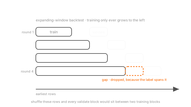
Cut chronologically instead, and backtest with an expanding or rolling window so you get several honest estimates rather than one. Then add a gap between train and validate whenever the label spans time: if the label is "did this churn within 30 days", the last 30 days of the training block overlap the validation period, and dropping them is the difference between a backtest and a rehearsal. Cross-validation schemes has the fold shapes.

The diagnosis is one command: re-split by date and compare. The gap between the two numbers was never yours.

A window that reaches forward while looking like a lag

Three ways this happens, all of them quiet.

rolling(3, center=True) averages the row either side. shift(-1) looks forward instead of back, and the minus sign is easy to type and impossible to see in a diff. And a rolling call applied to a frame that was sorted by customer_id rather than by timestamp computes a window over whatever order the rows happened to be in.

None of them error. The feature is numeric, plausibly distributed, and ranks well on importance, because it genuinely does contain information about the target — information from after the prediction moment.

Two habits catch all three. Sort by the event timestamp immediately after loading, and assert it. Then, for every window feature, check its value on the last row of your data: if it can be computed there, it only used the past, and if it comes back null or shifted, it was reaching forward.

The Quick Version

Ordering is the data. Rows aren't exchangeable, so a shuffle destroys what you were modelling.
Event time is when it happened, processing time is when you saw it, and a late arrival makes them disagree for good.
Resampling needs an aggregation rule per column: sum for counts, last for levels, mean for rates.
Lags, differences, rolling and expanding windows, calendar flags — every one strictly backwards from its own row.
Decompose into trend, seasonality and residual. Stationarity is a series whose mean and variance hold still, and differencing or a log gets you closer.
Adjacent rows are correlated, so your effective sample size is far below your row count and ordinary error bars are too narrow.
Split chronologically, backtest with an expanding or rolling window, and leave a gap whenever the label spans time.
A 3-period mean at one row was 12.67 trailing and 13.33 centred. The difference is tomorrow.