Diffusion Samplers

Why Does This Exist?

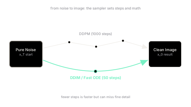
When Denoising Diffusion Probabilistic Models (DDPMs) first arrived, they produced incredible images but had a fatal flaw: speed. The mathematical formulation of a DDPM required traversing a Markov chain step-by-step. If the model was trained with 1,000 noise steps, you had to run the neural network exactly 1,000 times to generate a single image. While a Generative Adversarial Network (GAN) could spit out an image in 0.05 seconds, a DDPM could take 20 seconds.

Diffusion samplers (sometimes called schedulers or ODE solvers) were invented to decouple the training process from the generation process. Researchers realized that you don't actually have to walk the exact 1,000-step path the model was trained on. Instead, you can view the trained neural network as a continuous mathematical function (a vector field or differential equation) and use advanced numerical solvers to "skip" steps, getting to the same destination in 50, 20, or even 4 steps.

Think of It Like This

How It Actually Works

The breakthrough in diffusion sampling came when researchers realized that the discrete DDPM process could be reframed as a continuous Ordinary Differential Equation (ODE) or Stochastic Differential Equation (SDE). Once framed as an ODE, you can use a century's worth of numerical solver research (like Euler or Runge-Kutta methods) to solve it efficiently.

1. DDIM (Denoising Diffusion Implicit Models)

The first major leap was DDIM. The authors proved that the forward noise process didn't actually need to be a Markov chain (where step $t$ strictly depends on $t-1$). By making the process non-Markovian during inference, they derived a formula that allows you to skip steps. If a model was trained on $T=1000$, a DDIM sampler can evaluate the model at $t=1000, 950, 900, \dots, 0$. It achieved comparable quality in 50 steps to what DDPM achieved in 1,000. Furthermore, DDIM is deterministic: if you start with the same noise seed, you get the exact same image every time.

2. First-Order Solvers (Euler)

The simplest ODE solver is Euler's method. At a given noise level, the neural network predicts the direction to the clean image. An Euler sampler simply takes a straight-line step in that direction. Because the true path is curved, taking steps that are too large with Euler causes you to overshoot the curve, resulting in blurry or distorted images. It generally requires 30 to 50 steps for high quality.

3. Higher-Order Solvers (DPM-Solver, Heun)

To take even fewer steps without flying off the curve, we use higher-order solvers. A second-order solver (like Heun) evaluates the neural network, projects a step forward, evaluates the network again at that future point, and averages the two directions to take a perfectly curved step. Specialized solvers like DPM-Solver and DPM++ are mathematically optimized specifically for the diffusion ODE, allowing stunning image generation in as few as 10 to 20 steps.

4. Ancestral vs. Deterministic Samplers

You will often see samplers with an "a" at the end (e.g., Euler a). This stands for "ancestral." While deterministic solvers just move down the gradient, ancestral solvers actively inject a small amount of fresh random noise back into the image at every step, before denoising it again. This stochasticity can wash out artifacts and often results in more textured, "creative" images, though they will never converge to the exact same image twice, even with the same seed.

Show Me the Code

This code demonstrates a highly simplified inference loop using an Euler-style update rule, showing how we can skip steps by defining a custom schedule.

1import torch2
3def euler_sample(model, initial_noise, num_inference_steps=50, max_timesteps=1000):4    """5    A simplified Euler ODE solver for diffusion models.6    """7    device = initial_noise.device8    9    # Create a schedule of timesteps to evaluate (e.g., [1000, 980, 960, ..., 20])10    step_size = max_timesteps // num_inference_steps11    timesteps = torch.arange(max_timesteps, 0, -step_size, device=device)12    13    # Start with pure noise14    x = initial_noise15    16    for i, t in enumerate(timesteps):17        # 1. Ask the neural network to predict the noise in the current image18        t_tensor = torch.full((x.shape[0],), t, device=device)19        predicted_noise = model(x, t_tensor)20        21        # 2. Calculate the step size (dt)22        # In a real implementation, this incorporates the alpha/beta variance schedule23        dt = 1.0 / num_inference_steps24        25        # 3. Take a straight-line Euler step towards the clean image26        # x_{t-1} = x_t - direction * dt27        x = x - predicted_noise * dt28        29    return x30
31# Example usage:32# initial_noise = torch.randn(1, 3, 64, 64)33# clean_image = euler_sample(trained_unet, initial_noise, num_inference_steps=20)

Watch Out For

The Quick Version

• Generating an image with the original DDPM formula required 1,000 slow, sequential steps.
• Diffusion samplers treat the trained network as a continuous differential equation, allowing us to mathematically skip steps during inference.
• DDIM was the first major breakthrough, proving that the generative process could be deterministic and run in 50 steps.
• Higher-order ODE solvers (like DPM-Solver) calculate the curvature of the denoising path, allowing generation in as few as 10 to 20 steps.
• Ancestral samplers (like Euler a) inject fresh noise at every step, creating texture and variation, while deterministic samplers converge cleanly.

What to Read Next

• Read Score-Based Models to see the alternative continuous-time mathematical framework that proved diffusion models were just solving stochastic differential equations.
• Read Classifier-Free Guidance to understand how the prompt actually steers the sampler's path.