Gen AI

Hierarchical Navigable Small World (HNSW)

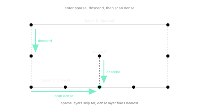
HNSW builds a multi-layered graph where top layers have long-distance links for fast skipping, and bottom layers have dense links for precise local search.

HNSW searches from the sparse top layer down to the dense bottom layer, quickly narrowing the search space before zooming in.

Why Does This Exist?

When dealing with massive datasets of high-dimensional vectors, finding the exact nearest neighbors using brute-force distance calculations becomes computationally impossible. This is known as the curse of dimensionality. To enable real-time search in vector databases and retrieval-augmented generation pipelines, we must trade perfect accuracy for speed.

Hierarchical Navigable Small World (HNSW) is currently the state-of-the-art algorithm for approximate nearest neighbor (ANN) search. It provides an exceptionally high recall rate (often above 95%) while maintaining sub-millisecond query latency. Unlike earlier tree-based approaches like KD-trees, which degrade quickly in high dimensions, HNSW scales beautifully. It achieves this by constructing a multi-layered graph structure inspired by skip lists and small-world network properties.

If you are using a modern vector database like Pinecone, Milvus, Qdrant, or Weaviate, the default index type powering your lightning-fast semantic searches is almost certainly an implementation of HNSW. Understanding how it builds and traverses its graph is essential for tuning its hyperparameters and balancing memory consumption against query speed.

Think of It Like This

Navigating the interstate highway system

Imagine you are driving from a small town in rural Montana to a specific address in downtown Miami. You don't take back roads the entire way.

First, you drive to the nearest interstate highway. The interstate is a "sparse" network—there are few exits, but it allows you to cross vast distances at high speed. You take the interstate all the way to Florida. This is the top layer of HNSW.

Once you reach the Miami area, you exit the interstate onto state highways and major arterial roads. The network becomes denser, the speed limit drops, but you are navigating closer to your specific neighborhood. This is the middle layer.

Finally, you turn onto local residential streets. This network is incredibly dense and interconnected. You navigate street by street until you arrive at the exact driveway. This is the bottom layer of HNSW. You found your destination quickly by skipping the dense local roads when you were far away, only descending into the dense network when you were close.

How It Actually Works

The Small World Property

HNSW builds upon the concept of Navigable Small World (NSW) graphs. In an NSW graph, nodes (vectors) are connected to a set of their nearest neighbors. The "small world" property means that most nodes are not connected to each other, but the average path length between any two nodes is very short (like the "six degrees of separation" concept). You can navigate the graph greedily: start at a random entry point, look at its neighbors, jump to the neighbor closest to your query vector, and repeat until you hit a local minimum where no neighbor is closer.

However, standard NSW has a scaling problem. As the graph grows, greedy routing takes too many hops.

Adding the Hierarchy

HNSW solves the scaling problem by introducing a hierarchy, drawing inspiration from probabilistic skip lists. The graph is split into multiple layers.

The bottom layer (Layer 0) contains every single vector in the dataset and is highly connected.
As you move up to Layer 1, Layer 2, etc., nodes are sampled probabilistically. Each successive layer contains exponentially fewer nodes.
The top layer contains only a handful of nodes and very long-range connections.

The Search Process

When a query vector arrives, the search begins at the very top layer.

Top-Down Routing: The algorithm finds the node closest to the query in the top layer using greedy search.
Descending: Once it finds the local minimum in the current layer, it uses that node as the entry point for the layer immediately below it.
Refining: Because the lower layer has more nodes, the search space is refined. The algorithm again routes greedily to the local minimum.
Base Layer Convergence: This process repeats until it reaches Layer 0. The search in Layer 0 explores the dense connections to find the absolute closest vectors, returning the top-k nearest neighbors.

Hyperparameters: M and ef

Two primary parameters govern HNSW's construction and performance:

M: The maximum number of bidirectional links created for every new element during insertion. A higher M creates a denser graph, which improves recall but increases memory usage and insertion time. Typical values range from 16 to 64.
ef (efConstruction and efSearch): The size of the dynamic candidate list used during routing. efConstruction controls how many entry points are explored when adding a new node (higher means a better quality graph but slower indexing). efSearch controls how many nodes are evaluated during the final query phase (higher means better recall but slower queries).

HNSW is entirely an in-memory algorithm. Every node's adjacency list and the vector itself must reside in RAM for the pointer-hopping to be fast. This makes it memory-hungry compared to compression-based algorithms like IVF-PQ, which is why hybrid approaches are becoming popular.

Show Me the Code

While writing a highly optimized HNSW implementation from scratch in Python is complex, we can use the industry-standard hnswlib library to see how the parameters are configured and how the index is queried.

1import hnswlib2import numpy as np3
4# Generate some dummy data5dim = 1286num_elements = 100007
8# Generating sample data9data = np.float32(np.random.random((num_elements, dim)))10query_data = np.float32(np.random.random((1, dim)))11
12# Declare the index13# space can be 'l2', 'ip' (inner product), or 'cosine'14index = hnswlib.Index(space='l2', dim=dim)15
16# Initialize the index17# max_elements: total capacity18# ef_construction: size of the dynamic list for the nearest neighbors (controls index quality)19# M: number of bidirectional links created for every new element20index.init_index(max_elements=num_elements, ef_construction=200, M=16)21
22# Add data to the index23# The IDs are simply integers from 0 to num_elements-124index.add_items(data, np.arange(num_elements))25
26# Set the search parameter27# ef controls the recall/speed tradeoff during querying28index.set_ef(50)29
30# Query the index for the top 3 nearest neighbors31labels, distances = index.knn_query(query_data, k=3)32
33print(f"Nearest neighbor IDs: {labels[0]}")34# -> Nearest neighbor IDs: [4213 8921 1045]35print(f"Distances: {distances[0]}")36# -> Distances: [1.234 1.456 1.789]

Watch Out For

Running out of RAM

Because HNSW relies on traversing a graph structure, it cannot easily page data out to a slow disk. The entire graph—including the raw vectors and all the bidirectional pointers—must stay in RAM. For billion-scale datasets, the memory overhead of the graph edges alone can become prohibitively expensive, forcing teams to move to IVF-PQ or quantized variants.

Stale connectivity after massive deletes

HNSW handles insertions beautifully, but deletions are notoriously difficult. When you delete a vector, the standard approach is to mark it as a "tombstone" (soft delete) rather than restructuring the graph. If you delete a large percentage of your database, the graph becomes riddled with tombstones, drastically slowing down search routing. You will eventually need to rebuild the index from scratch.

The Quick Version

Exact vector search scales terribly, so we use Approximate Nearest Neighbor (ANN) algorithms.
HNSW is the default ANN algorithm in modern vector databases because of its unmatched speed and high recall.
It works by building a multi-layered graph: sparse layers at the top for fast, long-distance jumps, and dense layers at the bottom for precise local search.
The tradeoff is high memory usage, as the entire graph structure of vectors and pointers must be kept in RAM.