Bias-Variance Decomposition

Test error splits into three piles: how wrong your model family is on average, how much it wobbles between training sets, and noise no model can remove.

Three fits scatter around their mean while the mean sits on the truth, so the error is all variance and noise with no bias

Why Does This Exist?

Your model nails training and flops on new data, or it flops on both. Those are different diseases with opposite cures, and guessing wrong costs you a week: more capacity fixes one and worsens the other. The decomposition tells you which patient you have by splitting expected squared error into three named piles, each responding to a different treatment.

This page proves the split and works it on numbers. The conceptual tradeoff, when to add capacity and when to regularize, lives in bias-variance tradeoff. The summaries it leans on are in expectation, variance and covariance.

The one idea you need first

Expected error averages over fresh training sets, not one lucky fit. Draw a dataset, fit, measure squared error at a fixed test point, repeat many times, average. Bias is how far the average prediction lands from truth. Variance is how much individual fits scatter around that average.

Think of It Like This

Three archers, one target

Three archers each loose one arrow at the same bullseye. Their arrows land left, center-left and far left: tightly grouped but off the mark. That group has high bias and low variance, so you adjust the sight, not the archers.

Next round the arrows land left, right and center: centered on average but scattered. Bias is near zero and variance is large, so you steady the archers instead. And if a gusty wind blows, some scatter stays whatever you do. That leftover is the noise.

Where it stops: real models cannot re-shoot the training set at will, so you estimate these piles with cross-validation rather than measuring them directly.

How It Actually Works

Fix a test input $x$ with truth $f(x)$ and noisy labels $y = f(x) + \epsilon$ , where $\epsilon$ has mean zero and variance $\sigma^2$ . Fit $\hat{f}$ on a random training set. The expected squared error splits cleanly:

\mathbb{E}\left[(y - \hat{f}(x))^2\right] = \underbrace{\left(f(x) - \mathbb{E}[\hat{f}(x)]\right)^2}_{\text{squared bias}} + \underbrace{\mathbb{E}\left[(\hat{f}(x) - \mathbb{E}[\hat{f}(x)])^2\right]}_{\text{variance}} + \underbrace{\sigma^2}_{\text{noise}}

In plain words: $\mathbb{E}$ averages over training sets, the first term punishes a systematically wrong model family, the second punishes a jumpy fitting procedure, and $\sigma^2$ is label noise nobody can fit. The cross term vanishes because $\epsilon$ has mean zero and is independent of the fit.

So complexity moves the first two terms in opposite directions. Richer families bend closer to truth (bias falls) but chase sampling quirks harder (variance climbs). The sum is U-shaped, which is why both tiny and huge models can flop.

Worked example

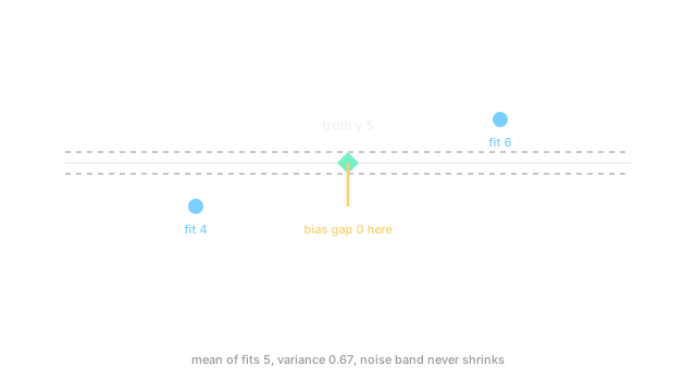
Truth $f(x) = 5$ with noise variance $\sigma^2 = 0.25$ . Three training sets produce predictions $\hat{f}$ of $4$ , $5$ and $6$ .

Mean prediction: $(4 + 5 + 6)/3 = 5$ . Bias: $5 - 5 = 0$ , so squared bias is $0$ . Variance: $((4-5)^2 + (5-5)^2 + (6-5)^2)/3 = (1 + 0 + 1)/3 \approx 0.67$ . Expected error: $0 + 0.67 + 0.25 = 0.92$ .

Zero bias, yet error $0.92$ . Every bit of it comes from wobble plus noise, so adding capacity cannot help: the family already centers on truth. More data or averaging (bagging) attacks the $0.67$ ; nothing attacks the $0.25$ .

Code

Averaging independent fits kills variance but not bias, and this snippet shows exactly that on the worked numbers.

1import numpy as np2
3
4def decomposition(fits: np.ndarray, truth: float, noise_var: float) -> tuple[float, float, float]:5    mean = float(fits.mean())  # average prediction across training sets6    bias2 = (truth - mean) ** 27    var = float(((fits - mean) ** 2).mean())8    return bias2, var, bias2 + var + noise_var9
10
11fits = np.array([4.0, 5.0, 6.0])12print(decomposition(fits, 5.0, 0.25))  # -> (0.0, 0.6667, 0.9167)

Three numbers out, matching the hand computation: bias squared $0$ , variance $0.67$ , total $0.92$ .

Watch Out For

Reading bias off a single fit

Symptom: one model predicts $4$ against truth $5$ and you declare bias $-1$ . Fix: bias is a property of the procedure's average, not one draw. That single $4$ could be an unbiased procedure's bad day (variance) rather than a systematically wrong family.

Chasing error below the noise floor

Symptom: validation error plateaus near your best estimate of label noise, yet training continues for days. Fix: estimate $\sigma^2$ first (repeated labels, annotator agreement). Error cannot go below it, and every further point of training loss is overfitting by definition.

The Quick Version

Expected squared error is squared bias plus variance plus irreducible noise, with no cross terms.
Bias measures the model family; variance measures the fitting procedure's wobble across datasets.
Complexity lowers bias and raises variance, so total error is U-shaped in capacity.
Averaging independent fits cuts variance and leaves bias untouched.
Noise is a floor: no model, however large, earns error below $\sigma^2$ .