Confounding and Selection Bias

A third variable can fake a treatment effect, and filtering on the wrong variable can fake one too, so causal claims need the graph, not just data.

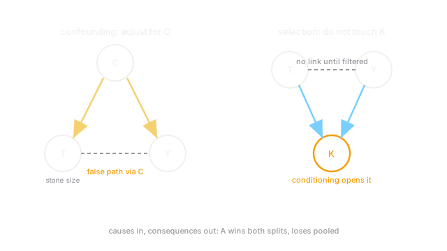
A confounder feeds both treatment and outcome creating a false path, while conditioning on a collider connects two causes that were independent

Why Does This Exist?

Coffee correlates with heart disease in raw data, yet the effect shrinks after accounting for smoking: smokers drink more coffee, and smoking harms the heart. The coffee-heart link was mostly a confounder at work. Hospital data shows the mirror trap: two independent conditions look negatively linked among the admitted, because admission itself favors having at least one. That is selection (collider) bias: filtering on a shared consequence manufactures association.

Both errors survive infinite data, so bigger samples never cure them. Only the causal graph tells you which variables to adjust for and which to leave alone. This page teaches the two graphs, the adjustment rule for each, and a Simpson-paradox table where the pooled and split answers disagree in sign.

The one idea you need first

A causal graph draws arrows for direct effects. A confounder $C$ points at both treatment $T$ and outcome $Y$ ( $T \leftarrow C \rightarrow Y$ ): a backdoor path. A collider $K$ receives from both ( $T \rightarrow K \leftarrow Y$ ): blocked by default, opened by conditioning.

Think of It Like This

Umbrellas, rain, and wet floors

Wet floors correlate with umbrella sales. The confounder is rain: it drives both. Blaming umbrellas for wet floors is confounding, fixed by comparing dry days to dry days and rainy days to rainy days.

Now consider only buildings with wet floors (selection). Among those, umbrella sightings and burst pipes look negatively linked: knowing nobody carried an umbrella raises the odds of a burst pipe, since something wet the floor. Neither causes the other; restricting to wet floors (a collider both can cause) manufactured the link. The fix is to stop filtering, not to adjust harder.

How It Actually Works

Confounding. The crude contrast $\mathbb{E}[Y \mid T=1] - \mathbb{E}[Y \mid T=0]$ mixes the treatment effect with $C$ 's influence. The backdoor fix stratifies: $\sum_c (\mathbb{E}[Y \mid T=1, c] - \mathbb{E}[Y \mid T=0, c]) P(c)$ . Weight each stratum's effect by its population share.

Collider bias. $T$ and $Y$ independent, but both raise admission $K$ . Among the admitted ( $K = 1$ ), $T$ and $Y$ correlate: learning $T = 0$ makes $Y = 1$ likelier, since something caused admission. The fix is to not condition on $K$ , or to model the selection explicitly.

Worked example

Kidney-stone treatments (the classic Simpson table). Treatment A: $273/350 \approx 78\%$ overall. Treatment B: $289/350 \approx 83\%$ overall. B looks better pooled. Split by stone size: small stones A $81/87 \approx 93\%$ vs B $234/270 \approx 87\%$ ; large stones A $192/263 \approx 73\%$ vs B $55/80 \approx 69\%$ . A wins in both groups. The reversal happens because doctors gave B mostly to easy small-stone cases ( $270$ small vs $80$ large) and A mostly to hard ones: stone size confounds treatment assignment. Stratified effect: A beats B by about $5$ points per group, weighted by group sizes.

Code

1def rate(n: int, d: int) -> float:2    return round(n / d, 3)  # plain success rate3
4
5# Pooled: B looks better.6print(rate(273, 350), rate(289, 350))  # -> 0.78 0.8267# Small stones: A wins 0.931 vs 0.867.8print(rate(81, 87), rate(234, 270))  # -> 0.931 0.8679# Large stones: A wins 0.73 vs 0.688.10print(rate(192, 263), rate(55, 80))  # -> 0.73 0.688

Pooled B wins by $4.6$ points; stratified A wins by $6.4$ and $4.2$ points. The pooled answer is the confounded one.

Watch Out For

Adjusting for a collider to fix confounding

Faced with bias, the reflex is to control for more variables. Controlling for a collider (or its descendant) creates association along a path that was blocked. Before adding a covariate, draw its arrows: adjust for shared causes, never for shared consequences.

Pooling heterogeneous groups without checking

Any pooled contrast can reverse after stratification when group assignment correlates with treatment. If treatment shares differ across groups by more than about twofold (here $270/80$ vs $87/263$ ), distrust the pooled number until you see the split table.

The Quick Version

Confounders feed treatment and outcome, faking effects through the backdoor path.
Conditioning on a collider connects independent causes, manufacturing association.
Fix confounding by stratifying on shared causes; fix selection by not filtering on consequences.
Kidney data: B wins pooled $83\%$ vs $78\%$ but A wins both splits ( $93\%$ vs $87\%$ , $73\%$ vs $69\%$ ).
Treatment imbalance across groups (here threefold) flags a pooled reversal.
Draw arrows before adjusting: causes in, consequences out.