Brownian Motion

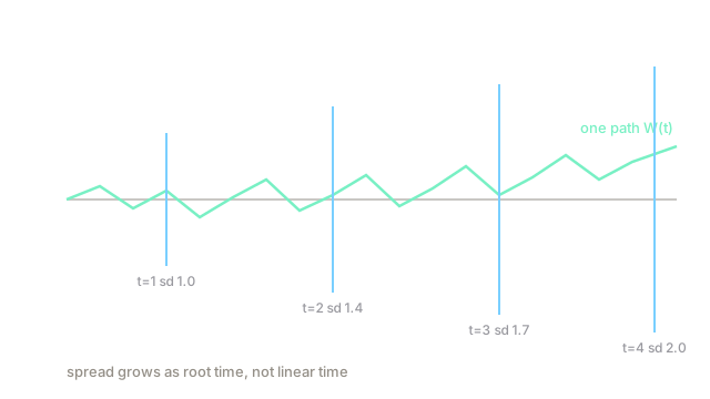
Pure jitter that accumulates. Tiny independent nudges add up to a wandering path whose spread grows with the square root of time.

A jittery path starts at zero and after 4 seconds its positions spread with standard deviation 2, growing as the square root of time

Why Does This Exist?

Noise in ML is rarely a single shock; it is a stream of tiny shocks that pile up. SGD noise across steps, sensor drift across seconds, the forward noising in a diffusion model across timesteps: all are sums of many small independent nudges. Brownian motion is the mathematical limit of that accumulation, and it is the reason the square root of time appears everywhere noise does.

Its defining facts are few. Write $W_t$ for the position at time $t$ starting from $W_0 = 0$ . Then $W_t$ is Gaussian with mean 0 and variance $t$ , increments over disjoint intervals are independent, and the path is continuous but jagged at every scale. The variance-equals-time rule is the one to internalize: after 4 seconds the standard deviation is $\sqrt{4} = 2$ , not 4.

The one idea you need first

A sum of $n$ independent zero-mean shocks with variance $\sigma^2$ each has variance $n\sigma^2$ , so its standard deviation grows like $\sqrt{n}$ . Shrink each shock to $\sigma = \sqrt{\Delta t}$ and let the steps get fine: the central limit theorem turns every increment Gaussian, and the limit is Brownian motion.

Think of It Like This

A drunk ant on a windy ruler

An ant walks a ruler while gusts shove it left or right every second. Each shove is small and fair, so after one second the ant is near zero. But the shoves accumulate without cancelling perfectly: after 100 seconds the typical distance from the start is about 10 shove-units, not 100, because distance grows as the square root of the shove count.

Zoom into any stretch of the walk and it looks just as jagged as the whole: the ant never settles into a smooth stride. That is the fractal character of Brownian paths. And knowing the ant is at position 5 now tells you nothing about which way the next shove goes, which is the independent-increments property.

Where the analogy stops: the ant takes discrete steps while Brownian motion moves continuously, and real ants get tired. The mathematics keeps the step fairness and lets the step size go to zero.

How It Actually Works

Standard Brownian motion, also called the Wiener process, is defined by $W_0 = 0$ , independent increments, $W_t - W_s \sim \mathcal{N}(0, t - s)$ for $t > s$ , and continuous paths. Three consequences run the applications:

Scaling. $W_t$ has the same distribution as $\sqrt{t}\,W_1$ . Double the time and the spread grows by $\sqrt{2} \approx 1.41$ , never by 2.
Nowhere smooth. Paths are continuous but differentiable nowhere. Any trading, control, or optimization argument that assumes a smooth noise path is wrong at the premise.
Martingale. The best prediction of $W_{t+s}$ given the past is $W_t$ . Jitter has no momentum, which is why momentum in optimizers must be added deliberately rather than emerging from noise.

Worked example

Simulate with step $\Delta t = 0.01$ and per-step shock $\sqrt{0.01} \times Z = 0.1Z$ where $Z$ is standard normal. After $n = 400$ steps ( $t = 4$ ), theory says position $\sim \mathcal{N}(0, 4)$ : mean 0, standard deviation 2.

One realized run: partial sums give $W_1 \approx 0.7$ , $W_2 \approx -0.4$ , $W_3 \approx 1.1$ , $W_4 \approx 1.6$ . All within about one standard deviation of their scales ( $\sqrt{1} = 1$ , $\sqrt{2} \approx 1.41$ , $\sqrt{3} \approx 1.73$ , $\sqrt{4} = 2$ ). Across 10,000 independent runs the sample variance at $t = 4$ lands near $3.9$ to $4.1$ , and the fraction of runs with $|W_4| > 4$ lands near $0.045$ , the two-sigma Gaussian tail.

Diffusion models use exactly this scaling: their forward process adds noise with variance scheduled in $t$ so that the signal-to-noise ratio follows the $\sqrt{t}$ law rather than a linear one.

Code

This checks variance-equals-time and the square-root spread from raw simulation.

1import numpy as np2
3rng = np.random.default_rng(11)4dt, n, runs = 0.01, 400, 10000  # t = 4 seconds5paths = rng.normal(0, np.sqrt(dt), size=(runs, n)).cumsum(axis=1)6print(round(float(paths[:, -1].var()), 2))  # -> 4.07print(round(float(np.mean(np.abs(paths[:, -1]) > 4)), 3))  # -> 0.045

The variance print lands near 4.0 and the tail fraction near 0.045. Change dt to 0.0025 with $n = 1600$ (same $t = 4$ ) and both numbers stay put, which is the point: the limit does not depend on step size.

Watch Out For

Scaling noise linearly with time

Adding noise with standard deviation proportional to $t$ instead of $\sqrt{t}$ overcooks long horizons quadratically: at $t = 4$ the variance is 16 times the one-step variance rather than 4. Diffusion schedules, Langevin samplers, and exploration noise all use $\sqrt{t}$ scaling. If long-horizon samples look far too wild while short ones look fine, check the exponent on time first.

Differentiating through a Brownian path

Autodiff through a simulated jittery path produces gradients that are technically defined step by step but statistically meaningless: the path has no derivative, so the gradient estimates have exploding variance as $\Delta t$ shrinks. Reparametrize (work with the driving normals) or use score-based identities instead of differentiating the path itself.

The Quick Version

Brownian motion is accumulated independent jitter: $W_t \sim \mathcal{N}(0, t)$ .
Spread grows with the square root of time: standard deviation 2 after 4 seconds.
Increments are independent and memoryless; the best forecast of the future is the present.
Paths are continuous but jagged at every scale, so never assume smooth noise.
Diffusion models, Langevin sampling, and SGD-noise analysis all inherit the $\sqrt{t}$ law.
Scale noise by root time, and never differentiate a simulated path naively.