Stochastic Gradient Descent Variants

Stochastic gradient descent estimates the true dataset gradient from tiny random mini-batches, using momentum and adaptive coordinate scaling to accelerate training.

Trajectories of vanilla SGD, SGD with momentum, RMSprop, and Adam navigating an elongated ravine toward the loss minimum.

Why Does This Exist?

In classical batch gradient descent, computing a single parameter update requires evaluating the loss gradient across every single training example in the dataset. If your dataset contains $N = 10,000,000$ images, taking one optimization step requires ten million forward passes and ten million backward passes through the neural network. Training would grind to an absolute halt.

Stochastic Gradient Descent (SGD) solves this bottleneck through random sampling: instead of computing the true full-batch gradient over all $N$ examples, it computes an unbiased gradient estimate over a small mini-batch of $B$ samples (typically $32$ to $512$ ). This accelerates iteration throughput by factors of thousands.

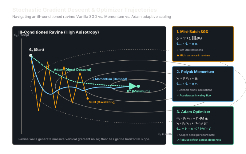
However, mini-batch estimation introduces substantial gradient variance (noise) and struggles with ill-conditioned loss landscapes. In narrow loss ravines where curvature is steep along one parameter axis and shallow along another, vanilla SGD ricochets violently between the steep ravine walls while making negligible progress along the gentle valley floor.

To overcome this, an evolutionary family of optimizer variants emerged: Momentum adds physical inertia to cancel out oscillating noise, RMSprop normalizes updates by historical gradient magnitudes, and Adam synthesizes momentum and adaptive variance scaling into the modern default optimizer for deep learning.

For the fundamentals of directional derivatives and loss slopes, see our guide on gradients.

Think of It Like This

A ping-pong ball vs. a heavy bowling ball with studded snow treads

Imagine trying to roll a ball down a steep, icy half-pipe ravine to reach the exit at the bottom. The sides of the half-pipe rise sharply to your left and right, but the ravine floor tilts only gently forward toward the finish line.

Vanilla SGD is like a lightweight ping-pong ball buffeted by erratic wind gusts (mini-batch noise). When you release it, gravity yanks it down the steep side wall. Because it has no mass or memory, it shoots straight across the floor and ricochets wildly up the opposite wall. It bounces endlessly back and forth across the ravine, traveling miles laterally while advancing only inches forward down the floor.

SGD with Momentum turns the ping-pong ball into a heavy bowling ball. Lateral bounces cancel each other out across steps, while consistent forward gravitational pull accumulates velocity, barreling smoothly down the center of the half-pipe.

Adam equips that bowling ball with intelligent motorized treads on each coordinate: it automatically applies brakes along the steep bouncing axis while hitting the gas pedal along the gentle, quiet forward axis.

The analogy stops because physical bowling balls obey continuous Newtonian physics in 3 dimensions with constant gravitational acceleration, whereas neural optimizers operate in discrete steps across non-Euclidean parameter landscapes.

How It Actually Works

From Mini-Batch SGD to Adaptive Moments

Given total training dataset $\mathcal{D} = \{(\mathbf{x}_i, y_i)\}_{i=1}^N$ and model parameter vector $\mathbf{\theta} \in \mathbb{R}^d$ , the true loss is the empirical expectation:

\mathcal{L}(\mathbf{\theta}) = \frac{1}{N} \sum_{i=1}^N \ell(f(\mathbf{x}_i; \mathbf{\theta}), y_i)

1. Mini-Batch Stochastic Gradient Descent

At step $t$ , we draw a random mini-batch $\mathcal{B}_t \subset \{1, \dots, N\}$ of size $B = |\mathcal{B}_t|$ . The mini-batch gradient $\mathbf{g}_t$ is:

\mathbf{g}_t = \frac{1}{B} \sum_{i \in \mathcal{B}_t} \nabla_{\mathbf{\theta}} \ell(f(\mathbf{x}_i; \mathbf{\theta}_t), y_i)

The stochastic update is:

\mathbf{\theta}_{t+1} = \mathbf{\theta}_t - \eta \mathbf{g}_t

Because samples are chosen uniformly at random, $\mathbf{g}_t$ is an unbiased estimator of the true gradient: $\mathbb{E}[\mathbf{g}_t] = \nabla \mathcal{L}(\mathbf{\theta}_t)$ . However, its covariance matrix scales inversely with batch size: $\text{Cov}(\mathbf{g}_t) \propto \frac{1}{B} \mathbf{\Sigma}$ .

2. Polyak Momentum

To suppress variance and accelerate through ravines, Polyak momentum introduces a velocity vector $\mathbf{v}_t \in \mathbb{R}^d$ governed by friction coefficient $\beta \in [0.9, 0.99]$ :

\mathbf{v}_t = \beta \mathbf{v}_{t-1} + \mathbf{g}_t, \quad \mathbf{\theta}_{t+1} = \mathbf{\theta}_t - \eta \mathbf{v}_t

Expanding this recurrence reveals an exponential moving average of past gradients:

\mathbf{v}_t = \sum_{\tau=1}^t \beta^{t-\tau} \mathbf{g}_\tau

Along oscillating axes, gradients flip signs ( $+g, -g, +g$ ), summing toward zero. Along consistent directions, gradients reinforce each other, multiplying the effective step size by $\frac{1}{1 - \beta}$ (a $10\times$ acceleration when $\beta = 0.9$ ).

3. RMSprop (Root Mean Square Propagation)

In anisotropic landscapes, different parameters require drastically different learning rates. RMSprop maintains an exponential moving average of the squared gradients $\mathbf{s}_t$ :

\mathbf{s}_t = \beta_2 \mathbf{s}_{t-1} + (1 - \beta_2) \mathbf{g}_t^2

where $\mathbf{g}_t^2$ denotes element-wise squaring. The update normalizes the step coordinate-wise:

\mathbf{\theta}_{t+1} = \mathbf{\theta}_t - \frac{\eta}{\sqrt{\mathbf{s}_t} + \epsilon} \odot \mathbf{g}_t

where $\odot$ denotes element-wise multiplication and $\epsilon \approx 10^{-8}$ prevents division by zero. Parameters with large historical gradients are scaled down; parameters with tiny gradients are amplified.

4. Adam (Adaptive Moment Estimation)

Adam combines the first moment (momentum) and second raw moment (RMSprop) while introducing crucial initialization bias corrections:

\mathbf{m}_t = \beta_1 \mathbf{m}_{t-1} + (1 - \beta_1) \mathbf{g}_t \quad (\text{first moment})

\mathbf{v}_t = \beta_2 \mathbf{v}_{t-1} + (1 - \beta_2) \mathbf{g}_t^2 \quad (\text{second moment})

Because $\mathbf{m}_0 = \mathbf{0}$ and $\mathbf{v}_0 = \mathbf{0}$ , both vectors are biased toward zero at early steps. Unbiasing yields:

\hat{\mathbf{m}}_t = \frac{\mathbf{m}_t}{1 - \beta_1^t}, \quad \hat{\mathbf{v}}_t = \frac{\mathbf{v}_t}{1 - \beta_2^t}

The final parameter update is:

\mathbf{\theta}_{t+1} = \mathbf{\theta}_t - \frac{\eta}{\sqrt{\hat{\mathbf{v}}_t} + \epsilon} \odot \hat{\mathbf{m}}_t

Standard hyperparameter defaults are $\beta_1 = 0.9$ , $\beta_2 = 0.999$ , and $\epsilon = 10^{-8}$ .

Worked Example

Let us compute the first step ( $t = 1$ ) of the Adam optimizer by hand.

Given parameters $\mathbf{\theta}_0 = [1.0, 2.0]^T$ , learning rate $\eta = 0.1$ , $\beta_1 = 0.9$ , $\beta_2 = 0.999$ , and $\epsilon = 10^{-8}$ . Suppose the observed gradient at $t = 1$ is severely ill-conditioned:

\mathbf{g}_1 = \begin{bmatrix} 0.2 \\ 4.0 \end{bmatrix}

The slope along $\theta_2$ is twenty times steeper than along $\theta_1$ .

First moment update ( $\mathbf{m}_0 = \mathbf{0}$ ):
$\mathbf{m}_1 = 0.9(0) + (1 - 0.9) \begin{bmatrix} 0.2 \\ 4.0 \end{bmatrix} = \begin{bmatrix} 0.02 \\ 0.40 \end{bmatrix}$
Second moment update ( $\mathbf{v}_0 = \mathbf{0}$ ):
$\mathbf{g}_1^2 = \begin{bmatrix} 0.2^2 \\ 4.0^2 \end{bmatrix} = \begin{bmatrix} 0.04 \\ 16.00 \end{bmatrix}$ $\mathbf{v}_1 = 0.999(0) + (1 - 0.999) \begin{bmatrix} 0.04 \\ 16.00 \end{bmatrix} = \begin{bmatrix} 0.00004 \\ 0.01600 \end{bmatrix}$
Bias correction at step $t = 1$ :
$1 - \beta_1^1 = 1 - 0.9 = 0.1 \implies \hat{\mathbf{m}}_1 = \frac{\mathbf{m}_1}{0.1} = \begin{bmatrix} 0.2 \\ 4.0 \end{bmatrix}$ $1 - \beta_2^1 = 1 - 0.999 = 0.001 \implies \hat{\mathbf{v}}_1 = \frac{\mathbf{v}_1}{0.001} = \begin{bmatrix} 0.04 \\ 16.00 \end{bmatrix}$
Effective parameter update:
$\sqrt{\hat{\mathbf{v}}_1} = \begin{bmatrix} \sqrt{0.04} \\ \sqrt{16.00} \end{bmatrix} = \begin{bmatrix} 0.2 \\ 4.0 \end{bmatrix}$ $\frac{\hat{\mathbf{m}}_1}{\sqrt{\hat{\mathbf{v}}_1} + \epsilon} = \begin{bmatrix} \frac{0.2}{0.2} \\ \frac{4.0}{4.0} \end{bmatrix} = \begin{bmatrix} 1.0 \\ 1.0 \end{bmatrix}$ $\mathbf{\theta}_1 = \mathbf{\theta}_0 - \eta \begin{bmatrix} 1.0 \\ 1.0 \end{bmatrix} = \begin{bmatrix} 1.0 \\ 2.0 \end{bmatrix} - 0.1 \begin{bmatrix} 1.0 \\ 1.0 \end{bmatrix} = \begin{bmatrix} 0.9 \\ 1.9 \end{bmatrix}$

Notice the outcome: even though the raw gradient along $\theta_2$ was $20\times$ larger than along $\theta_1$ , Adam normalized both displacement components to $1.0$ , completely neutralizing the ill-conditioned ravine on step 1!

Code

1import numpy as np2
3
4class AdamOptimizer:5
6    def __init__(7        self,8        lr: float = 0.1,9        beta1: float = 0.9,10        beta2: float = 0.999,11        eps: float = 1e-8,12    ) -> None:13        self.lr = lr14        self.beta1 = beta115        self.beta2 = beta216        self.eps = eps17        self.m: np.ndarray | None = None18        self.v: np.ndarray | None = None19        self.t = 020
21    def step(self, theta: np.ndarray, grad: np.ndarray) -> np.ndarray:22        if self.m is None:23            self.m = np.zeros_like(theta)24            self.v = np.zeros_like(theta)25
26        self.t += 127        # Update biased 1st and 2nd moment estimates28        self.m = self.beta1 * self.m + (1.0 - self.beta1) * grad29        self.v = self.beta2 * self.v + (1.0 - self.beta2) * (grad**2)30
31        # Compute bias-corrected moments32        m_hat = self.m / (1.0 - self.beta1**self.t)33        v_hat = self.v / (1.0 - self.beta2**self.t)34
35        # Apply adaptive update36        theta_next = theta - self.lr * m_hat / (np.sqrt(v_hat) + self.eps)37        return theta_next38
39
40# Test on ill-conditioned gradient41opt = AdamOptimizer(lr=0.1)42theta_0 = np.array([1.0, 2.0])43grad_1 = np.array([0.2, 4.0])44
45theta_1 = opt.step(theta_0, grad_1)46print(f"Step 1 theta: {theta_1}")47# -> Step 1 theta: [0.9 1.9]48
49# Verify step 2 with alternating gradient sign50grad_2 = np.array([0.2, -3.8])51theta_2 = opt.step(theta_1, grad_2)52print(f"Step 2 theta: {theta_2}")53# -> Step 2 theta: [0.8 1.90481546]

Watch Out For

Omitting Adam's bias correction during warm-up

Failing to implement Adam's bias corrections ( $\hat{\mathbf{m}}_t = \mathbf{m}_t / (1 - \beta_1^t)$ and $\hat{\mathbf{v}}_t = \mathbf{v}_t / (1 - \beta_2^t)$ ) is a severe implementation error.

Because $\mathbf{v}$ is initialized at zero and $\beta_2 = 0.999$ , the second moment without correction at step $t=1$ is $\mathbf{v}_1 = 0.001 \mathbf{g}_1^2$ . Dividing by $\sqrt{\mathbf{v}_1} = \sqrt{0.001} |\mathbf{g}_1| \approx 0.0316 |\mathbf{g}_1|$ produces an effective step scale roughly $\frac{1}{\sqrt{0.001}} \approx 31.6$ times larger than intended! This uncalibrated spike destabilizes transformers and language models in their opening steps.

Fix: Always apply exact bias-corrected estimates $\hat{\mathbf{m}}_t$ and $\hat{\mathbf{v}}_t$ , and pair Adam with a learning rate warm-up schedule over the first 500 to 2,000 steps of training.

The Quick Version

Mini-batch SGD computes unbiased gradient estimates over subsets of size $B$ , trading per-step precision for massive data throughput.
Momentum accumulates past velocity vectors with decay $\beta$ , damping high-frequency lateral oscillations and accelerating through ravines.
RMSprop divides updates by the root mean square of historical gradients, equalizing step sizes across parameters with mismatched scales.
Adam combines first-moment momentum with second-moment variance scaling and exact bias correction, providing the standard robust optimizer for deep architectures.
Always use learning rate warm-up schedules when training deep networks with Adam to prevent early gradient variance from destabilizing attention layers.