Math

The Chain Rule

When one thing feeds into another, you find the total effect by multiplying the effects along the path — which is exactly how a network learns which of its early weights to blame.

$To find how the final loss responds to a weight three steps upstream, read the local slope off every arrow along the path and multiply them together; that product is the whole of backpropagation$

To find how the final loss responds to a weight three steps upstream, read the local slope off every arrow along the path and multiply them together; that product is the whole of backpropagation

Why Does This Exist?

A neural network's first layer never touches the loss. It feeds the second layer, which feeds the third, which eventually produces a number that gets compared against a label. So when the loss comes out too high, how do you work out how much of that was the first layer's fault?

You cannot measure it directly — the loss has no idea the first layer exists. The chain rule is the answer, and it is the reason deep learning is possible at all: backpropagation is this rule, applied over a computational graph. Not analogous to it, not inspired by it. It is this rule, plus bookkeeping.

It also explains a piece of history. Deep networks were known to be more expressive long before they could be trained, and the chain rule shows why. A path through 30 layers multiplies 30 local slopes together. If each one is around 0.5, the product is about $10^{-9}$ — the first layer receives essentially no signal. Every architectural fix you have heard of for that problem, from careful initialisation to residual connections, is a fix for a product of numbers being the wrong size.

The one idea you need first

A derivative is a rate: if $\partial a / \partial z = 12$ , then nudging $z$ moves $a$ about twelve times as much. That is the only prerequisite, and this page is about what happens when you have several of those rates in a row.

Think of It Like This

Three currency exchanges in a row

You want to know how many yen you get per pound. Nobody at the counter quotes that rate, but three people quote rates that chain: pounds to dollars at 1.25, dollars to euros at 0.90, euros to yen at 160.

You do not add these. You multiply: $1.25 \times 0.90 \times 160 = 180$ yen per pound. Each rate converts the units of the one before it, and the units cancel down the chain until only yen-per-pound is left.

Two things fall straight out of this picture. A single bad rate ruins the whole conversion, no matter how good the others are — that is the vanishing gradient. And if you already know the pounds-to-dollars rate, you can reuse it for any onward chain rather than recomputing it, which is why backpropagation caches its intermediate results instead of starting over for every weight.

How It Actually Works

If $L$ depends on $a$ , and $a$ depends on $w$ , then the rate at which $L$ responds to $w$ is the product of the two local rates:

\frac{\partial L}{\partial w} = \frac{\partial L}{\partial a} \cdot \frac{\partial a}{\partial w}

In plain words: how much the loss moves per unit of $a$ , times how much $a$ moves per unit of $w$ . The notation is doing you a favour here — it looks like the $\partial a$ terms cancel like fractions, and while that is not a proof, it is a reliable way to remember the shape.

Longer chains just keep multiplying. For $w \to z \to a \to L$ :

\frac{\partial L}{\partial w} = \frac{\partial L}{\partial a} \cdot \frac{\partial a}{\partial z} \cdot \frac{\partial z}{\partial w}

So the recipe is mechanical, and worth stating as a procedure because that is how it is implemented:

Forward pass. Compute each intermediate value in order, keeping them. You will need them.
Local derivatives. At each step, differentiate that step alone with respect to its own input. Local means local: differentiating $a = z^2$ needs no knowledge of what produced $z$ or what consumes $a$ .
Multiply back. Start from $\partial L / \partial L = 1$ at the output and walk backwards, multiplying by each local derivative as you pass it.

Step 3 is why it is called backpropagation: one number, the accumulated product so far, is handed backwards from layer to layer. Each layer multiplies it by its own local derivative and passes it on. No layer ever needs to know the whole network.

Why the direction matters

You could equally walk the chain forwards, and that is a real technique — forward-mode differentiation. It loses on cost, decisively, and the reason is worth knowing.

Forward mode gets you the derivative of everything with respect to one input. Reverse mode gets you the derivative of one output with respect to everything. Training has millions of inputs (the parameters) and exactly one output (the scalar loss). So reverse mode gets the entire gradient in one backward sweep, while forward mode would need one sweep per parameter. For a 7-billion-parameter model that is the difference between a single pass and seven billion of them.

Multiple paths add

One caveat that catches people out. When a variable influences the output through more than one route, the chain rule gives you a contribution along each route, and the contributions add:

\frac{\partial L}{\partial w} = \sum_{\text{paths } p} \left( \prod_{\text{edges } e \in p} \frac{\partial\, \text{out}_e}{\partial\, \text{in}_e} \right)

In plain words: multiply along each path, then sum across paths. This is not an exotic case — it is what weight sharing is, so it applies to every convolution filter, every recurrent step, and every tied embedding.

Worked example

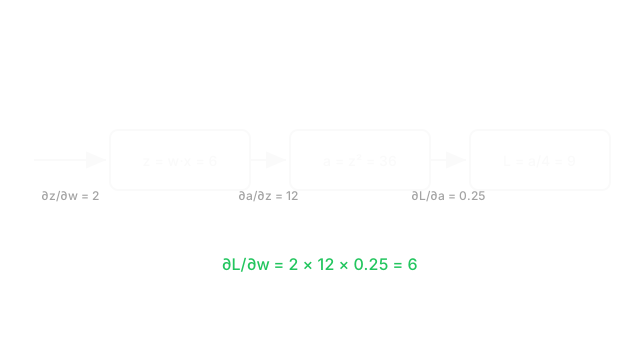
Take a two-step composition with $x = 2$ fixed and a weight $w = 3$ :

z = w x, \qquad a = z^2, \qquad L = \tfrac{1}{4}a

Forward: $z = 6$ , then $a = 36$ , then $L = 9$ .

Now the three local derivatives, each computed from its own step in isolation:

$\partial z / \partial w = x = 2$
$\partial a / \partial z = 2z = 12$ — note this needs the forward value $z = 6$ , which is why the forward pass is kept
$\partial L / \partial a = \tfrac{1}{4} = 0.25$

Multiply them: $0.25 \times 12 \times 2 = 6$ .

Worth checking independently, because a chain-rule answer is easy to get subtly wrong. Substituting everything gives $L = (wx)^2/4 = 4w^2/4 = w^2$ , so $\partial L/\partial w = 2w = 6$ . The chain agreed.

Show Me the Code

1import numpy as np2
3
4def forward_backward(w: float, x: float) -> tuple[float, float]:5    z = w * x            # scalars throughout; shapes would be (1,) as arrays6    a = z**27    loss = 0.25 * a8    # Walk back from the output, multiplying local derivatives as we go.9    d_a = 0.25           # dL/da10    d_z = d_a * 2 * z    # dL/dz — reuses the cached forward value z11    d_w = d_z * x        # dL/dw12    return loss, d_w13
14
15def numeric(w: float, x: float, h: float = 1e-5) -> float:16    f = lambda v: 0.25 * (v * x) ** 217    return (f(w + h) - f(w - h)) / (2 * h)18
19
20print(forward_backward(3.0, 2.0))                            # -> (9.0, 6.0)21print(np.isclose(forward_backward(3.0, 2.0)[1], numeric(3.0, 2.0)))  # -> True

Nine and six, matching the hand calculation. The d_z line is the one to stare at: it multiplies the accumulated derivative by a local one and uses a value saved during the forward pass. Those two facts together are why training a large model needs so much memory — every intermediate activation is held until the backward pass consumes it.

Watch Out For

Dropping a path when a variable is used twice

Write $L = f(w) \cdot g(w)$ and it is easy to differentiate one factor, get an answer, and stop. But $w$ reaches $L$ by two routes, so the true derivative is the sum of both path contributions — this is the product rule, which is the chain rule with two paths.

In practice this shows up in hand-written custom layers, and it is a nasty bug because the result is not obviously broken. You get a gradient of the right shape and roughly the right magnitude, pointing in a slightly wrong direction. Training still works, just worse than it should, and nobody suspects the derivative.

Weight sharing is the same trap at scale: a tied embedding matrix used at both the input and the output layer receives gradient from both, and summing only one of them is silently wrong. This is the single strongest argument for running a numerical gradient check on any derivative you derived yourself.

Assuming a long product will behave

Thirty layers means thirty factors multiplied together, and products of many numbers are numerically unforgiving in a way sums are not.

Average factor 0.5 over 30 layers gives roughly $10^{-9}$ : the early layers receive a gradient indistinguishable from zero and simply stop learning. That is the vanishing gradient problem. Average factor 1.5 gives about $1.9 \times 10^{5}$ , and in float16 — whose maximum is about 65,504 — the result overflows to infinity, which then poisons every parameter it touches with NaN.

The uncomfortable part is how narrow the safe band is. Factors need to sit near 1.0 on average, and staying there is not automatic; it is what careful initialisation, normalisation layers, and residual connections are all buying. If a deep model produces NaN a few hundred steps in, suspect this product before you suspect your data.

The Quick Version

The chain rule multiplies local rates along a path to get the total rate. Backpropagation is this rule over a graph.
Each step's derivative is computed in isolation, which is what lets layers be written independently of each other.
Forward values must be cached, because local derivatives usually need them. That is the memory cost of training.
Reverse mode wins because training has millions of parameters and one scalar loss.
Several paths to the same variable means multiply along each, then add — weight sharing and the product rule are this case.
A product of many factors vanishes below 1 and explodes above it. Most deep-learning architecture tricks exist to keep it near 1.