Multivariable Chain Rule

When one input reaches the output through several routes at once, multiply along each route and add the routes up. That sum is the whole of backpropagation.

With t feeding z through x and y, the top route contributes 8 times 4 and the bottom 12 times 3, and the total rate 68 is their sum

Why Does This Exist?

The single-variable chain rule handles chains: A feeds B feeds C. But real models are trees, not chains. A parameter feeds two layers that later recombine. A hidden state feeds every future step of a recurrence. An embedding matrix is read at the input and again at the output. In each case one input reaches the loss through several routes at once, and the single-chain formula silently drops all but one of them.

The multivariable chain rule fixes exactly that. It says: multiply along each route, then add across routes. Backpropagation over any computational graph is this rule executed mechanically, which makes it the single most-run equation in deep learning.

The one idea you need first

A partial derivative $\partial z / \partial x$ measures the response of $z$ to $x$ with every other input frozen. The multivariable rule is built from these frozen readings plus the rates at which the frozen variables themselves move. If partials are fuzzy, reread that page first, because every term below is one.

Think of It Like This

Two roads into town, counted separately

Commuters reach downtown by the bridge or by the tunnel, and you want the total flow per minute. You would never count one road and declare the job done. You count the bridge rate, count the tunnel rate, and add.

Derivatives through a tree work the same way. Each route from input to output carries its own product of local rates, and the total rate is the sum over routes. A shared upstream variable is a commuter hub serving several roads: busy on each, and the total is all of them. Forgetting a route undercounts exactly the way ignoring the tunnel would.

The analogy stops at linearity. Traffic on one road slows the other, but derivative routes add cleanly with no interference. The sum is exact, not an approximation, which is why the rule can be trusted inside an optimizer loop running millions of times.

How It Actually Works

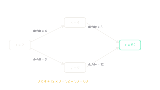
Suppose $z$ depends on $x$ and $y$ , and both depend on $t$ . The total rate of $z$ with respect to $t$ is:

\frac{dz}{dt} = \frac{\partial z}{\partial x}\frac{dx}{dt} + \frac{\partial z}{\partial y}\frac{dy}{dt}

In plain words: the $x$ route contributes its product, the $y$ route contributes its product, and the answer is both. Note the notation doing its job: $\partial z / \partial x$ is partial because $z$ has another input, while $dx / dt$ is ordinary because $x$ depends only on $t$ .

With more variables the pattern extends by summation, and in matrix form the sum becomes a Jacobian product. A layer with 1,000 inputs and 1,000 outputs chains through a $1000 \times 1000$ matrix of partials, and reverse-mode differentiation multiplies by it from the left so one backward sweep serves all parameters.

Worked example

Take $z = x^2 + y^2$ with $x = t^2$ and $y = 3t$ , evaluated at $t = 2$ .

Forward values first: $x = 4$ , $y = 6$ , $z = 16 + 36 = 52$ .

Now each route. The $x$ route: $\partial z / \partial x = 2x = 8$ and $dx / dt = 2t = 4$ , giving $8 \times 4 = 32$ . The $y$ route: $\partial z / \partial y = 2y = 12$ and $dy / dt = 3$ , giving $12 \times 3 = 36$ . Total: $32 + 36 = 68$ .

Check it independently by substituting first: $z(t) = t^4 + 9t^2$ , so $dz/dt = 4t^3 + 18t = 32 + 36 = 68$ . The tree agreed. Dropping either route would have answered 32 or 36, both wrong, which is the entire pitfall below.

Code

The snippet computes the tree answer and checks it against a finite difference, the same gradient-check habit the gradients page recommends.

1def forward_backward(t: float) -> tuple[float, float]:2    x = t**23    y = 3 * t4    z = x**2 + y**25    dz_dt = 2 * x * 2 * t + 2 * y * 3  # one product per route, then add6    return z, dz_dt7
8
9def numeric(t: float, h: float = 1e-5) -> float:10    f = lambda v: (v**2) ** 2 + (3 * v) ** 211    return (f(t + h) - f(t - h)) / (2 * h)12
13
14z, dz = forward_backward(2.0)15print((z, dz))                        # -> (52.0, 68.0)16print(abs(dz - numeric(2.0)) < 1e-6)  # -> True

Fifty-two and sixty-eight, matching the hand calculation. The dz_dt line is the rule in code: each term pairs a frozen partial with the rate of its own variable.

Watch Out For

Summing only the route you remembered

When a variable is used twice, every hand derivation risks counting one use. The result has the right shape and roughly the right size, pointing slightly wrong, so training merely underperforms and nobody suspects the derivative. Weight tying, residual adds, and recurrent steps all create multi-route variables at scale. Any derivative you derived yourself, check numerically.

Writing partial d where the total belongs

$\partial z / \partial t$ is meaningless here because $z$ is not directly a function of $t$ alone, and $dz/dt$ is the quantity training needs. Mixing the two notations in a derivation is how terms quietly go missing: a partial where a total belongs drops every indirect route. Read each symbol as a question. Partial asks one input while the rest sit still. Total asks everything that moves.

The Quick Version

One input reaching the output through several routes contributes along every route, and the contributions add.
Each route contributes a product of local rates: frozen partials times single-variable rates.
In matrix form the sum becomes a Jacobian product, which is what layers chain through.
Reverse mode wins for training because one scalar loss fans out to millions of parameters.
Dropping a route gives a plausible wrong gradient, so check hand-derived trees numerically.