Math

Computational Graphs

Every operation your model performs is recorded as a node in a one-way network, and training works by walking that network backwards — which is also why training eats so much memory.

A framework records every operation as a node in a directed acyclic graph, runs it forward caching each value, then walks the same graph in reverse to accumulate gradients

Why Does This Exist?

You write four lines of Python and call .backward(), and correct gradients appear for every parameter. Nobody derived them. There is no symbolic differentiation step you can inspect. What happened?

A graph happened. While your forward code ran, the framework was recording — every operation became a node, every data dependency became an edge, and every intermediate value was stashed at the node that produced it. .backward() walks that recording in reverse.

This is the page that explains three things you otherwise have to accept on faith. Why training needs several times more memory than inference — the forward pass is holding everything for the backward pass. Why gradient checkpointing trades compute for memory and what it actually discards. And why an in-place operation can silently corrupt your gradients: it overwrites a value the graph was keeping.

The chain rule says backpropagation is that rule "applied over a computational graph". This is the graph.

Think of It Like This

A kitchen that keeps every intermediate bowl

A chef follows a recipe: chop onions, fry them, add stock, blend, season. A one-way sequence, each step consuming what the last produced.

Now the chef must answer a question after serving: "if I had used 10% more onion, how much saltier would the final dish have tasted?" Answering it requires walking backwards through every step, and at each one asking how sensitive that step's output was to its input. But the sensitivity of the blending step depends on how much liquid was in the pot at that moment — you cannot reason about it from the recipe alone. You need the actual state.

So the chef keeps every intermediate bowl. Nothing gets washed until the question is answered. That is the memory cost of training, and it is not optional: the sensitivity of squaring a number depends on the number.

Gradient checkpointing is the chef keeping only every fourth bowl and re-cooking the missing steps when needed. Less shelf space, more cooking.

How It Actually Works

A computational graph is a DAG where each node is an operation and each edge carries a value from producer to consumer. Leaf nodes are inputs and parameters; the single root is usually the scalar loss.

It is a graph in the exact technical sense, and being acyclic is what makes everything work: a DAG has a topological order, so the operations can be sequenced with every input ready before it is needed.

Two passes over one structure

Forward. Traverse in topological order, computing each node's output and caching it at the node. This produces the loss, and it leaves the graph decorated with every intermediate value.

Backward. Traverse in reverse topological order, starting from $\partial \mathcal{L} / \partial \mathcal{L} = 1$ at the root. At each node, multiply the incoming gradient by that node's local derivative and pass the result to its inputs. When a node feeds several consumers, its incoming gradients sum — which is the multiple-paths rule from the chain rule, implemented as accumulation.

Each node only needs to know how to differentiate itself. That locality is why you can write a custom layer without touching the optimiser, and why frameworks ship thousands of ops rather than one giant derivative.

Static versus dynamic graphs

Two designs, and the distinction still shapes the tooling:

Static (define-then-run) — build the whole graph up front, then feed data through. Early TensorFlow. The compiler sees everything, so it can fuse and optimise aggressively, but control flow that depends on data is awkward and debugging is indirect.
Dynamic (define-by-run) — the graph is recorded fresh on every forward pass, as ordinary Python executes. PyTorch. Python if and while just work, stack traces point at your code, and each iteration may have a different graph.

Dynamic won on ergonomics, and then the gap closed from the other side: torch.compile traces a dynamic graph and hands it to a compiler, recovering static-graph optimisation. Understanding that graph capture is happening is what makes its failure modes legible — a data-dependent branch forces a graph break, which is why some code compiles to one fast kernel and some silently falls back.

Where the memory goes

Here is the accounting that matters in practice. Peak training memory is roughly:

\text{parameters} + \text{gradients} + \text{optimizer state} + \text{activations}

The first three scale with parameter count. The fourth scales with parameters × batch size × sequence length, and it is the one that surprises people, because it is often the largest term and it exists only because of the backward pass.

That is why inference needs a fraction of training's memory: no graph is retained, so activations are freed as soon as they are consumed. torch.no_grad() is precisely the instruction "do not record", and forgetting it in an evaluation loop is one of the most common out-of-memory causes there is.

Gradient checkpointing is the direct trade. Keep activations only at chosen checkpoints; during the backward pass, recompute the discarded segments from the nearest checkpoint. Memory drops from $O(n)$ to about $O(\sqrt{n})$ in the number of layers, at the cost of roughly one extra forward pass — commonly quoted as about 30% more time for a large memory saving. It is a graph-level trade, and it only makes sense once you see the graph.

Worked example

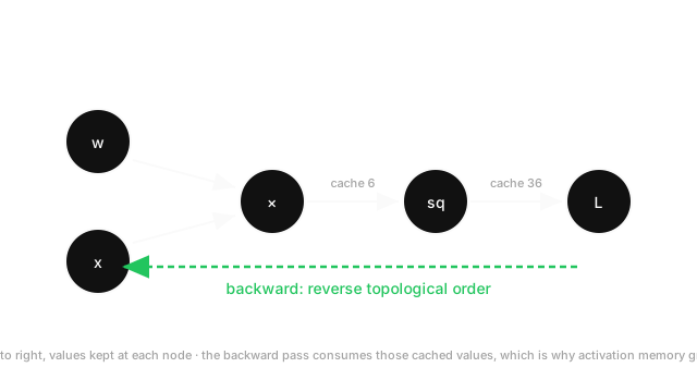
Take the graph in the diagram: $w = 3$ , $x = 2$ , then $z = w \cdot x$ , $a = z^2$ , $\mathcal{L} = a / 4$ .

Forward, in topological order. $z = 3 \times 2 = 6$ , cached at the multiply node. $a = 6^2 = 36$ , cached at the square node. $\mathcal{L} = 36/4 = 9$ .

Backward, in reverse order. Start at the root with $\partial \mathcal{L} / \partial \mathcal{L} = 1$ .

Divide node: local derivative $1/4$ , so $\partial \mathcal{L} / \partial a = 1 \times 0.25 = 0.25$ .
Square node: local derivative $2z = 12$ — and this needs the cached $z = 6$ . So $\partial \mathcal{L} / \partial z = 0.25 \times 12 = 3$ .
Multiply node: local derivative with respect to $w$ is $x = 2$ . So $\partial \mathcal{L} / \partial w = 3 \times 2 = 6$ .

Verify independently: substituting gives $\mathcal{L} = (wx)^2/4 = w^2$ , so $\partial \mathcal{L} / \partial w = 2w = 6$ . Agreed.

The line to stare at is the square node. Its local derivative was $2z$ , a number that only existed because the forward pass ran. Overwrite that cached 6 and the backward pass computes a wrong gradient with no error raised. That is the in-place bug, made concrete.

Show Me the Code

1import numpy as np2
3
4class Tape:5    """A three-node graph, recorded forward and replayed backward."""6
7    def forward(self, w: float, x: float) -> float:8        self.x, self.z = x, w * x        # cache z: the backward pass needs it9        self.a = self.z**210        return 0.25 * self.a11
12    def backward(self) -> float:13        d_a = 0.25                        # dL/da14        d_z = d_a * 2 * self.z            # dL/dz  <- uses the CACHED z15        return d_z * self.x               # dL/dw16
17
18tape = Tape()19print(tape.forward(3.0, 2.0), tape.backward())   # -> 9.0 6.020
21# Corrupt the cache the way an in-place op would. No error, wrong gradient.22tape.forward(3.0, 2.0)23tape.z = 999.024print(tape.backward())                            # -> 999.0, silently wrong

Nine and six match the hand calculation. The last two lines are the whole warning: nothing raised, and the gradient is nonsense.

Watch Out For

Retaining the graph in an evaluation loop

Every forward pass builds a graph and holds activations for a backward pass that, during evaluation, never comes. Run validation without torch.no_grad() and memory climbs with every batch until the process dies.

It is easy to write, because the evaluation loop looks like the training loop minus .backward() — and the missing piece is invisible. Worse, a small validation set finishes before memory runs out, so the bug ships and appears later when the set grows or the batch size changes.

The related version is accumulating metrics wrongly. total_loss += loss keeps a reference to the loss tensor, which keeps its whole graph alive, so you retain one graph per batch for the entire epoch. total_loss += loss.item() extracts a plain float and lets the graph be freed. That single missing .item() is one of the most common memory leaks in ML code.

Wrap evaluation in torch.no_grad() (or torch.inference_mode(), which is stricter and slightly faster), and detach anything you store.

Modifying a tensor the graph is still holding

In-place operations — x += y, x.relu_(), x[mask] = 0 — overwrite memory that a cached node may still need. When the backward pass reaches that node, the value it relies on is gone.

PyTorch catches many of these with a version counter and raises RuntimeError: one of the variables needed for gradient computation has been modified by an inplace operation. That error is a gift: it is loud, and it names the problem. The dangerous cases are the ones the counter misses, where you get a wrong gradient and a model that trains slightly worse for no visible reason.

The temptation is real, because in-place saves memory and memory is exactly what you are short of. The rule of thumb: in-place is safe on a tensor that is not needed for any backward computation — typically the output of an operation whose derivative does not depend on its output. relu_() is usually fine because ReLU's gradient depends only on the sign. Squaring is not, because its derivative is $2z$ .

When in doubt, write the out-of-place version and let the framework's memory planner handle it. And if a gradient looks subtly wrong, run a numerical gradient check before suspecting anything else.

The Quick Version

A computational graph is a DAG: nodes are operations, edges carry values, the root is the scalar loss.
Forward pass traverses topological order and caches each node's output. Backward pass traverses the reverse.
Each node differentiates only itself. Gradients from multiple consumers are summed at a node.
Being acyclic is what guarantees a topological order exists, and therefore that this works at all.
Static graphs optimise better; dynamic graphs debug better. torch.compile traces a dynamic graph to get both.
Activation memory exists purely to serve the backward pass, and it scales with batch and sequence length. This is why training needs far more memory than inference.
Gradient checkpointing keeps fewer activations and recomputes the rest: about $O(\sqrt{n})$ memory for roughly one extra forward pass.
torch.no_grad() for evaluation, and .item() when accumulating metrics. Both prevent retained graphs.
In-place operations can overwrite a cached value the backward pass needs.