Math

Computational Complexity for ML

Counting operations tells you how a cost grows; counting bytes moved tells you how long it actually takes — and in machine learning the second one usually wins.

Below a certain amount of arithmetic per byte fetched, a kernel spends its time waiting for memory and never reaches the chip's advertised speed, however many operations you remove

Why Does This Exist?

You halve the number of operations in a kernel and it runs no faster. You increase the batch size eightfold and throughput goes up more than eightfold. Neither makes sense under a pure operation count, and both are routine.

The reason is that modern accelerators can do arithmetic far faster than they can fetch data. A GPU might sustain hundreds of teraflops while its memory delivers a couple of terabytes per second — a ratio of a hundred or more operations per byte. Feed it a kernel that does less arithmetic per byte than that and the arithmetic units sit idle waiting, and no amount of removing operations helps.

So the useful question is not "how many operations" but "how many operations per byte moved". That single reframing explains why batching pays, why FlashAttention was a breakthrough without changing the maths, why quantisation speeds up inference beyond the memory saving, and why a decoder generating one token at a time is so inefficient.

This is also the page behind the complexity questions in interviews: stating $O(n^3)$ for a matmul is the entry fee, and knowing when that number is irrelevant is the actual answer.

Think of It Like This

A fast chef and a slow corridor

A chef can chop vegetables extraordinarily quickly. The ingredients are in a storeroom down a long corridor, and each trip takes a while.

Give the chef one carrot per trip and the kitchen's output is set entirely by walking speed. The chopping is instant; the corridor is everything. Buy a faster knife and nothing changes.

Give the chef a whole crate per trip and the picture flips. Now they spend most of their time chopping, the corridor barely matters, and a faster knife genuinely helps.

The deciding quantity is how much chopping happens per trip. Below some threshold you are corridor-limited; above it, knife-limited. And the threshold is a property of the kitchen, not of the recipe.

Accelerators are exactly this. The corridor is memory bandwidth, the knife is the arithmetic units, and the threshold is a fixed ratio for each chip. Most of performance engineering in ML is arranging to carry crates instead of carrots — which is what batching, fusion, and tiling all do.

How It Actually Works

Two costs, always count both.

Arithmetic — the operation count, what big-O usually describes.

Memory traffic — the bytes moved between slow memory and the compute units.

Their ratio is the arithmetic intensity:

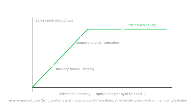
I = \frac{\text{operations}}{\text{bytes moved}}

Each chip has a threshold ratio, its peak flops divided by its peak bandwidth. Below it you are memory-bound; above it, compute-bound. That is the roofline in the diagram: a rising line where bandwidth limits you, and a flat ceiling where arithmetic does.

Matrix multiplication, both ways

An $n \times n$ by $n \times n$ product does about $2n^3$ operations and moves about $3n^2$ numbers — read both inputs, write the output. So:

I = \frac{2n^3}{3n^2 \cdot \text{bytes}} = \frac{2n}{3 \cdot \text{bytes}}

Intensity grows with $n$ . Large matmuls are compute-bound and hit near-peak throughput. Small or thin ones are memory-bound and run at a fraction of peak no matter how fast the chip is.

That is the whole reason batching works. Multiplying one $1 \times 768$ input by a $768 \times 3072$ weight matrix reads the entire weight matrix — 2.4 million numbers — to do very little arithmetic. Stack 32 inputs and you read the same weights once for 32 times the work. The weights were going to be fetched either way, so the extra rows are nearly free.

Attention, and why FlashAttention mattered

For sequence length $n$ and head dimension $d$ , attention computes $QK^{T}$ ( $n^2 d$ operations), a softmax over $n^2$ entries, then multiplies by $V$ (another $n^2 d$ ). So arithmetic is $O(n^2 d)$ — quadratic in sequence length, which is the well-known scaling problem.

The less-quoted problem is memory. The score matrix has $n^2$ entries, and at $n = 4096$ that is 16.7 million numbers per head — 33.5 MB in float16. With 32 heads, over a gigabyte, written to and read back from slow memory.

FlashAttention changed no mathematics. It computes attention in tiles that fit in fast on-chip memory and never materialises the full score matrix, using the log-sum-exp trick to combine tiles' softmaxes correctly. Same $O(n^2 d)$ operations, dramatically less memory traffic, and a large real speedup. It is the clearest possible demonstration that operation counts are the wrong thing to optimise.

Where the costs actually are

Worth knowing by shape rather than by memorising:

Dense layer, batch $b$ , dims $d_{\text{in}} \to d_{\text{out}}$ : $2 b\, d_{\text{in}} d_{\text{out}}$ operations. Compute-bound when $b$ is large, memory-bound at $b = 1$ .
Attention: $O(n^2 d)$ operations, $O(n^2)$ memory unless tiled.
Brute-force nearest neighbour: $O(nd)$ per query, and entirely memory-bound — you read the whole index to do one pass of arithmetic. This is why approximate indexes exist.
Autoregressive generation: one token at a time means $b = 1$ per step, so decoding is memory-bound and reads every weight for each token. That is why the KV cache, speculative decoding, and continuous batching all exist — they raise the arithmetic intensity of a fundamentally bandwidth-limited operation.
Training costs roughly three times a forward pass: forward, backward with respect to inputs, backward with respect to weights.

Why quantisation is faster than the flop count suggests

Halving the bit width halves the bytes moved. In a memory-bound regime, time is set by bytes, so you get close to a 2× speedup even if the arithmetic runs at the same rate. For autoregressive decoding — memory-bound by construction — this is most of why int8 and int4 inference is fast. The memory saving is not a side benefit; it is the mechanism.

Worked example

A dense layer with $d_{\text{in}} = 768$ and $d_{\text{out}} = 3072$ , weights in float16 (2 bytes).

The weight matrix holds $768 \times 3072 = 2{,}359{,}296$ numbers, so 4.7 MB must be read regardless of batch size.

Batch of 1. Operations $= 2 \times 1 \times 768 \times 3072 = 4.72$ million. Bytes moved $\approx 4.7$ MB. So:

I = \frac{4.72 \times 10^{6}}{4.72 \times 10^{6}} \approx 1 \text{ operation per byte}

Against a chip threshold of ~100, that is firmly memory-bound — roughly 1% of peak arithmetic throughput.

Batch of 128. Operations $= 2 \times 128 \times 768 \times 3072 = 604$ million. The weights are still read once; the activations add $128 \times 768 \times 2 = 0.2$ MB in and $128 \times 3072 \times 2 = 0.8$ MB out, so about 5.7 MB total:

I = \frac{6.04 \times 10^{8}}{5.7 \times 10^{6}} \approx 106 \text{ operations per byte}

Now compute-bound. Operations rose 128-fold while bytes rose only 1.2-fold, so intensity rose about 106-fold. This is why throughput improves superlinearly with batch size up to the point of saturation — and why it stops improving after.

The attention numbers, for contrast. At $n = 4096$ and $d = 64$ per head: about $2 \times 2 \times 4096^2 \times 64 \approx 4.3$ billion operations, against a score matrix of $4096^2 = 16.8$ million entries, or 33.5 MB in float16 — per head, written then read again. Thirty-two heads puts that over a gigabyte of avoidable traffic, and avoiding it is what FlashAttention does.

Show Me the Code

1def dense_cost(batch: int, d_in: int, d_out: int, bytes_per: int = 2) -> tuple[float, float]:2    ops = 2 * batch * d_in * d_out                      # multiply + add3    weights = d_in * d_out * bytes_per                   # read once, any batch size4    activations = (batch * d_in + batch * d_out) * bytes_per5    return ops, weights + activations6
7
8for b in (1, 8, 128, 1024):9    ops, byts = dense_cost(b, 768, 3072)10    print(b, f"{ops/1e6:9.1f}M ops", f"{byts/1e6:6.2f}MB", f"intensity {ops/byts:7.1f}")11# -> 1      4.7M ops  4.72MB  intensity     1.0   memory-bound12# -> 8     37.7M ops  4.78MB  intensity     7.913# -> 128  604.0M ops  5.70MB  intensity   106.0   compute-bound14# -> 1024 4831.8M ops 12.56MB intensity   384.715
16# Attention's hidden cost is the score matrix, not the operation count.17n, d, heads = 4096, 64, 3218scores_mb = n * n * 2 / 1e619print(round(scores_mb, 1), round(scores_mb * heads / 1000, 2))   # -> 33.6 1.07 (MB, GB)

The intensity of 1.0 at batch 1 and 106 at batch 128 match the hand calculation, and the jump is the batching argument in numbers. The last line is the gigabyte of score-matrix traffic that FlashAttention removes without changing a single operation.

Watch Out For

Optimising the operation count of a memory-bound kernel

Removing arithmetic from a kernel that is waiting on memory changes nothing, and this is where a great deal of optimisation effort goes to waste.

The classic case is a chain of small elementwise operations — a bias add, an activation, a dropout mask, a scale. Each has almost no arithmetic per element and each reads and writes the whole tensor, so the sequence is bandwidth-limited end to end. Making the activation function cheaper is invisible. Fusing the operations into one kernel so the tensor is read once and written once is a large win, and it removes no arithmetic at all.

The same logic explains why asymptotically faster matmul algorithms are rarely used. Strassen's $O(n^{2.807})$ removes operations while adding memory traffic and worse numerical behaviour, and on hardware where the arithmetic was not the bottleneck it loses.

The habit is to measure before optimising. Compute the arithmetic intensity of the kernel you care about and compare it against your hardware's ratio — that one number tells you which side you are on. Then profile: if the arithmetic units are idle, the answer is fusion, tiling, better layout, or a narrower dtype, not a cleverer formula.

Reading big-O as a prediction of runtime

Asymptotic complexity describes how cost grows. It says nothing about constants, memory behaviour, or cache locality, and in ML those often dominate at the sizes you actually run.

Two examples make the point. Two $O(n^2)$ implementations can differ by an order of magnitude purely from access pattern — a row-major traversal versus column-major on the same data. And a hand-written triple-loop matmul and a BLAS call are both $O(n^3)$ with a performance gap of a hundredfold or more, entirely from blocking and vectorisation.

The direction of the error is consistent: big-O flatters algorithms with poor locality. Sparse formats have excellent operation counts and irregular memory access, so a sparse matmul frequently loses to a dense one until sparsity is well past 90%. Practitioners are regularly surprised by this, and the surprise is always in the same direction.

So use big-O for what it is good at — deciding whether an approach can scale to your target size, and spotting the accidental quadratic in a data pipeline. Then benchmark at realistic sizes with realistic data, because crossover points are empirical. And when you quote a complexity in an interview, follow it with which resource is actually binding: that is the answer that shows you have run the thing.

The Quick Version

Count operations and bytes moved. Their ratio is arithmetic intensity.
Each chip has a threshold (peak flops over peak bandwidth). Below it you are memory-bound, above it compute-bound.
An $n\times n$ matmul is $2n^3$ operations against $3n^2$ numbers, so intensity grows with $n$ .
Batching works because the weights are read once regardless: batch 1 gives intensity ~1, batch 128 gives ~106.
Attention is $O(n^2 d)$ operations and $O(n^2)$ memory. At $n=4096$ the score matrix is 33.5 MB per head.
FlashAttention changed no maths — it tiles the computation so the score matrix is never materialised.
Autoregressive decoding runs at batch 1 per step, so it is memory-bound and reads every weight per token.
Quantisation gives close to a linear speedup in memory-bound regimes because time is set by bytes.
Training costs roughly 3× a forward pass.
Brute-force nearest neighbour is memory-bound, which is why approximate indexes exist.
Fusing elementwise chains is a large win and removes no arithmetic.
Big-O flatters algorithms with poor locality. Sparse often loses to dense below ~90% sparsity. Benchmark at real sizes.