Concentration of Measure

Well-behaved functions of many independent inputs barely wobble. Change one input and the output moves a little, so the whole function concentrates around its mean almost as tightly as a plain average.

Changing one of 500 inputs moves the output by at most a small step, so the whole distribution piles up in a narrow band around its mean

Why Does This Exist?

Averages concentrate, but learning never evaluates a plain average. Validation error is a complicated function of the whole training set, a spectral norm is a complicated function of a whole matrix, and a test metric is a complicated function of every example. Each one depends on hundreds of independent inputs through a nonlinear rule, so Hoeffding on a sum does not directly apply.

Concentration of measure extends the thin-tail promise from sums to well-behaved functions. If changing one input moves the output by at most $c_i$ (a bounded difference), the function behaves like an average with those step sizes. This is the tool that carries generalisation arguments: the gap between train and test error is a function of $n$ samples with small bounded differences, so it concentrates. Without it, every guarantee would stop at coin flips.

Prerequisite in one paragraph. You need a tail bound for sums, where $P$ denotes chance. Markov and Chebyshev inequalities give the slow version; sub-Gaussian variables give the fast exponential version used here. The central limit theorem describes the limiting shape while this page bounds the distance from the mean at finite samples.

Think of It Like This

An election decided by 500 precincts

No single precinct decides the national popular vote share. Flip one precinct and the total moves by at most its population weight, a fraction of a percent. Because every piece has small leverage, the final share lands in a narrow band around its expected value almost every time.

A concentrated function works the same way. Each input is one precinct with bounded leverage $c_i$ . Many small leverages mean a sharp total. The failure mode is also the same: give one precinct half the votes and the sharpness evaporates.

Where the analogy stops: precincts can correlate through turnout waves, and the theorem needs independence. Correlated inputs keep their leverage but lose the guarantee.

How It Actually Works

Let $f(X_1, \ldots, X_n)$ be a function of $n$ independent inputs. Say $f$ has bounded differences $c_1, \ldots, c_n$ , meaning swapping input $i$ for any alternative value changes $f$ by at most $c_i$ while all other inputs stay fixed. McDiarmid's inequality then says $P(|f - E[f]| \ge t) \le 2\exp(-2t^2 / \sum c_i^2)$ , where $E[f]$ is the mean of $f$ and $t$ is the deviation. Compare Hoeffding: same form, with $c_i$ playing the role of interval lengths.

The Gaussian cousin is cleaner. If $X$ is a standard Gaussian vector and $f$ is $L$ -Lipschitz, meaning $|f(x) - f(y)| \le L\lVert x - y\rVert$ for a constant $L$ (a slope cap), then $P(|f - E[f]| \ge t) \le 2\exp(-t^2 / 2L^2)$ . A 1-Lipschitz function of a high-dimensional Gaussian, like a normalised norm, fluctuates on a constant scale no matter the dimension. That is the precise sense in which high-dimensional space has no room for gradual transitions: sets expand and functions flatten.

Worked example

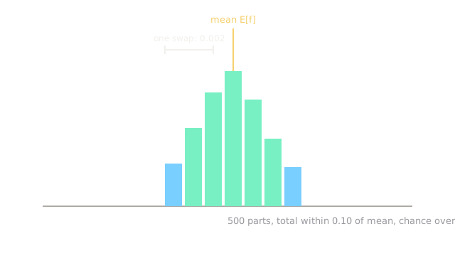
Take $n = 500$ parts, each able to shift a quality score in $[0, 1]$ by at most $c_i = 1/500 = 0.002$ when swapped. Then $\sum c_i^2 = 500 \times 0.000004 = 0.002$ . Ask for $t = 0.10$ . The exponent is $2 \times 0.01 / 0.002 = 0.02/0.002 = 10$ , so $P(|f - E[f]| \ge 0.10) \le 2\exp(-10) \approx 2 \times 0.0000454 = 0.0000908$ . The score sits within $0.10$ of its mean with chance above $0.9999$ .

Soften the claim to match the diagram caption: with $t = 0.07$ , the exponent is $2 \times 0.0049/0.002 = 4.9$ and $2\exp(-4.9) \approx 2 \times 0.00745 = 0.0149$ , chance above $0.985$ . Either way a 500-piece assembly with tiny individual leverage is nearly deterministic at the $0.10$ scale.

Watch Out For

Applying McDiarmid to a maximum with large leverage

The maximum over $n$ values has bounded differences $c_i$ as large as the whole range: swapping one input can install a new maximum. The sum $\sum c_i^2$ then stays order $n$ times a constant and the bound goes slack. People quote McDiarmid for a max and wonder why the guarantee is empty.

Fix: maxima need chaining or union bounds, not bounded differences. Check the worst-case swap before quoting the theorem.

Forgetting independence of the inputs

McDiarmid and Gaussian concentration both need independent inputs. Feed in 500 augmented copies of 50 base images and the effective $n$ is near 50, not 500. The bound computed with $n = 500$ claims sharpness the data cannot support, and the empirical spread proves it.

Fix: count independent sources, not rows. If rows share a base example, a batch or a patient, group them first.

The Quick Version

Concentration extends thin tails from averages to functions with small per-input leverage.
McDiarmid: swapping input $i$ moves $f$ by at most $c_i$ , then tails decay as $2\exp(-2t^2/\sum c_i^2)$ .
Lipschitz functions of Gaussians fluctuate on scale $L$ regardless of dimension.
With 500 parts each worth 0.002, the total stays within 0.10 of its mean with chance above 0.9999.
Maxima and dependent inputs break the leverage assumption, so check the worst swap and independence first.