The Condition Number

One number for how much a matrix amplifies errors: the ratio of its biggest stretch to its smallest. Large means fragile answers.

A circle entering a matrix with stretches 10 and 1 exits as a long thin ellipse, so errors along the stretched axis grow tenfold

Why Does This Exist?

Two systems can both be solvable yet differ wildly in trustworthiness. Nudge the inputs by a rounding error and one system's answer barely moves while the other's swings. The condition number

\kappa(A) = \frac{\sigma_{\max}}{\sigma_{\min}} = \lVert A \rVert_2 \lVert A^{-1} \rVert_2

measures that fragility: a relative wobble of $\epsilon$ in $b$ can exit $Ax = b$ amplified up to $\kappa(A) \cdot \epsilon$ in $x$ . A matrix with $\kappa = 10$ is mildly touchy; one with $\kappa = 10^{12}$ turns double precision into noise.

This number explains half of numerical linear algebra's behaviour: why the normal equations ( $X^T X$ squares the condition number) lose to QR, why feature standardisation speeds up solvers, and why the Hessian's eigenvalue spread in Jacobian and Hessian sets the learning-rate dilemma. Sizes come from norms; systems from linear systems and least squares.

The one idea you need first

Singular values are a matrix's independent stretch factors, largest $\sigma_{\max}$ to smallest $\sigma_{\min}$ . Along the top singular vector inputs grow the most; along the bottom they shrink the most. The condition number is the ratio between those extremes: how uneven the stretching is.

Think of It Like This

A photocopier with uneven zoom

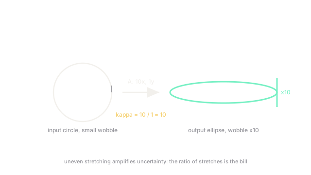
A photocopier enlarges horizontally by 10 and vertically by 1. Feed it a circle and a long thin ellipse comes out. Now smudge the input by a millimetre vertically: the output smudge is a millimetre. Smudge it horizontally: the output smudge is a centimetre.

Worse, run it backwards (solve the system): a millimetre of output smudge could have come from a tenth of a millimetre of input, or from a full millimetre, and the machine cannot tell you which. The zoom ratio 10 is the condition number: the factor by which uncertainty can grow when you invert. A copier with zoom 1 in both directions (orthogonal matrix, $\kappa = 1$ ) never amplifies anything.

How It Actually Works

The error bound that matters: for $Ax = b$ with perturbed $\tilde{b} = b + \Delta b$ ,

\frac{\lVert \Delta x \rVert}{\lVert x \rVert} \le \kappa(A)\,\frac{\lVert \Delta b \rVert}{\lVert b \rVert}

Relative input error times $\kappa$ bounds relative output error. Two consequences: forming $X^T X$ squares $\kappa$ (a $\kappa = 10^4$ problem becomes $10^8$ , borderline unsolvable in single precision), and preconditioning means finding $M$ such that $M^{-1}A$ has a smaller $\kappa$ before iterating.

Worked example

Take $A = \mathrm{diag}(1, 10)$ : stretches 1 and 10, so $\kappa = 10/1 = 10$ . Solve $Ax = b$ with $b = [1, 10]$ , giving $x = [1, 1]$ . Now perturb $b$ by $[0, 0.1]$ (a 1% relative wobble, since $\lVert b \rVert \approx 10.05$ ):

\Delta x = A^{-1}\Delta b = [0, 0.01], \quad \frac{\lVert \Delta x \rVert}{\lVert x \rVert} = \frac{0.01}{1.414} \approx 0.007

Here the wobble landed on the tame axis. Aim it at the fragile axis instead, $\Delta b = [0.1, 0]$ : $\Delta x = [0.1, 0]$ and the relative error hits $0.1/1.414 \approx 7\%$ from a 1% input. Same $\kappa$ , direction-dependent damage, worst case exactly $\kappa$ -fold. That direction dependence is why the bound uses $\le$ .

Code

The point is the check: compute $\kappa$ and confirm the determinant can look innocent while conditioning screams.

1import numpy as np2
3
4A = np.array([[1.0, 0.0], [0.0, 10.0]])5print(float(np.linalg.cond(A)))  # -> 10.06B = np.array([[1e6, 0.0], [0.0, 1e-6]])7print(float(np.linalg.det(B)))   # -> 1.08print(float(np.linalg.cond(B)))  # -> 1e+12

$B$ has determinant 1, the picture of health, and a condition number of a trillion. Determinants measure volume; conditioning measures unevenness. Never read one for the other.

Watch Out For

Trusting a determinant of one

As the code shows, $\det = 1$ coexists with $\kappa = 10^{12}$ : volume preserved, directions mangled. Determinants near zero do flag singularity, but moderate determinants say nothing about conditioning. Ask for $\kappa$ (or an estimate) whenever a solve must be trusted, not the determinant.

Training on unscaled features and blaming the optimiser

Features in units of millions beside features in thousandths build a design matrix with enormous $\kappa$ , and gradient descent crawls along the valley floor exactly as the Hessian's spread predicts. Standardise first: zero mean, unit variance. It is the cheapest preconditioner in machine learning, and skipping it disguises a conditioning problem as a tuning problem.

The Quick Version

$\kappa(A) = \sigma_{\max} / \sigma_{\min}$ : relative input error can grow $\kappa$ -fold in the answer.
The diag(1, 10) example scores 10: a 1% wobble can exit near 7% along the fragile axis.
Normal equations square $\kappa$ ; prefer QR or SVD on ill-conditioned problems.
Determinant 1 does not mean healthy: the $10^6$ / $10^{-6}$ diagonal has $\kappa = 10^{12}$ .
Standardise features first: it is preconditioning you get for free.