Probability Foundations
The rules for reasoning when you do not know the answer — how to combine chances, and what changes the moment you learn something new.
Why Does This Exist?
Supervised learning has a one-line definition that only makes sense once this page does: a classifier models the conditional distribution . It does not output a label. It outputs a belief about labels, given an input — and the vertical bar in that expression is conditional probability, which is the single most important idea here.
Get this wrong and a whole class of mistakes follows. Multiplying probabilities that are not independent is how naive Bayes earns the word "naive". Reading a 99%-accurate test as 99% certainty is the base-rate error that misprices risk in production. Treating a model's softmax output as a calibrated probability when it was trained to be confident is how teams ship systems that are wrong and sure about it.
None of this needs measure theory. It needs three rules and one habit: always ask conditional on what.
Think of It Like This
A dartboard you throw at blindfolded
Picture a wall with a dartboard painted on it, and you throw a dart at a random spot on the wall. The whole wall is everything that could happen. The chance of hitting any painted region is simply that region's share of the wall's area.
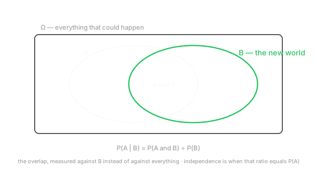
Now someone tells you the dart landed in the left half. You have not moved the dart, and nothing about the wall changed — but your question did. The left half is now the entire world you are reasoning inside, and the chance of the dart being on the dartboard is the dartboard's share of the left half, not of the wall.
That reframing is conditioning, and it explains the arithmetic. You divide by the probability of what you learned because you are re-measuring against a smaller world. If the dartboard happens to occupy the same fraction of the left half as it does of the whole wall, then learning "left half" told you nothing useful — and that is exactly what independence means.
How It Actually Works
Three objects, and you need all three.
The sample space is every outcome that could occur — six faces for a die, every real number for a temperature reading. An event is any subset of it: "the die shows an even number" is the subset . A probability assigns each event a number in such that and the probabilities of disjoint events add.
That is the whole foundation. Everything below is consequence.
The two combining rules
For "or", add and subtract the overlap:
In plain words: add the two chances, then remove the double-count where both happen. Skipping that subtraction is the most common arithmetic slip in the whole subject.
For "and", multiply — but the second factor must be conditional:
In plain words: the chance both happen is the chance happens, times the chance happens given that it did. Notice this is exact and always true. It is the definition of conditional probability rearranged, not an approximation.
Conditional probability
Rearranging the "and" rule gives the definition:
In plain words: of all the times happens, what fraction also has ? The denominator is the re-measuring — you have restricted the world to , so you divide by how big is. It requires : conditioning on something impossible is not a question with an answer.
Two things worth fixing in place now, because both cause real errors:
- and are different numbers. The probability of a positive test given illness is not the probability of illness given a positive test. Swapping them is so common it has a name, the prosecutor's fallacy, and Bayes' theorem exists to convert between them.
- Conditioning can move a probability either way. It is not "narrowing down" toward certainty. can be larger than, smaller than, or equal to .
Independence is a conclusion, not an assumption
and are independent exactly when learning one tells you nothing about the other:
The multiply-the-probabilities shortcut everyone remembers is only valid under independence. That is the caveat that gets dropped, and dropping it is how models become confidently wrong — see the second pitfall.
Joint, marginal, conditional
Three views of the same table of probabilities, and the vocabulary matters because papers use it constantly:
- Joint — both together.
- Marginal — one of them, ignoring the other, obtained by summing the joint over every value of the other. The name comes from literally totalling a table in its margin.
- Conditional — one of them once the other is known.
Machine learning lives in the third. A generative model learns the joint ; a discriminative model learns only the conditional and never models how inputs are distributed. That distinction is the whole difference between the two families.
Worked example
Roll a fair six-sided die. Let be "the roll is even" and be "the roll is 4 or higher".
, so . , so . The overlap , so .
Now condition:
In plain words: among rolls of 4 or more, two of the three are even. Learning raised the chance of from 0.5 to 0.667 — so these events are not independent. Check it against the product rule: , but . Not equal, so not independent, and multiplying 0.5 by 0.5 here would have been wrong.
Contrast that with = "the roll is 3 or higher", . Then , so , and . Equal — so and are independent, which is not obvious from looking at them. Independence is arithmetic, not intuition.
Code
from itertools import product
def prob(event, space: list[int]) -> float: return sum(1 for s in space if event(s)) / len(space)
die = [1, 2, 3, 4, 5, 6]is_even, at_least_4 = lambda r: r % 2 == 0, lambda r: r >= 4
p_a = prob(is_even, die) # 0.5p_b = prob(at_least_4, die) # 0.5p_ab = prob(lambda r: is_even(r) and at_least_4(r), die) # 2/6
print(round(p_a, 3), round(p_b, 3), round(p_ab, 3)) # -> 0.5 0.5 0.333print(round(p_ab / p_b, 3)) # -> 0.667 P(A|B)print(round(p_a * p_b, 3)) # -> 0.25 != 0.333, so dependent
# Two dice are genuinely independent, so here the product rule DOES hold.pairs = list(product(die, die))both = sum(1 for a, b in pairs if a % 2 == 0 and b >= 4) / len(pairs)print(round(both, 3), round(p_a * p_b, 3)) # -> 0.25 0.25Every number matches the hand calculation. The last two lines are the contrast worth keeping: the product rule failed for two events on one die and held for two events on separate dice.
Watch Out For
Reading the conditional backwards
is a property of the test. is what the patient wants to know. They are different numbers, and when the condition is rare they are wildly different — a 99%-accurate test for something affecting 1 in 10,000 people yields a positive result that is correct under 1% of the time.
This is not a trick question, it is a routine production error. Any time a monitoring system flags a rare event, the flag rate is dominated by false positives, and the same arithmetic applies to fraud detection, content moderation, and anomaly alerts. Teams build dashboards on the wrong direction of the conditional and then wonder why analysts stop trusting the alerts.
The habit that fixes it: whenever you see a percentage attached to a test or a classifier, say out loud which quantity it is conditional on. If you cannot, you do not yet know what the number means. Converting between the two directions requires the base rate, and that is what Bayes' theorem does.
Multiplying probabilities that are not independent
is a special case, not a rule. The general form always has a conditional in it, and using the shortcut on dependent events produces a number that is confidently and often enormously wrong.
Naive Bayes is the honest example — it assumes every feature is independent given the class, multiplies through, and is called "naive" precisely because that is false. Words in a document are heavily correlated, so the products are badly miscalibrated. It still classifies acceptably because the ranking survives even when the probabilities do not, which is a useful and frequently misunderstood distinction.
Where it genuinely bites is anywhere you multiply a chain of estimates and report the result as a probability: the reliability of a multi-step pipeline, the chance an agent completes a five-tool task, a compound risk estimate. Failures in those systems are strongly correlated — one bad retrieval causes the next bad generation — so the true joint probability is much worse than the product suggests. If you must multiply, say plainly that you are assuming independence, and treat the answer as a bound rather than an estimate.
The Quick Version
- The sample space is everything that could happen; an event is a subset; probabilities of disjoint events add.
- For "or": add, then subtract the overlap. Forgetting the subtraction double-counts.
- For "and": . Always true, and the definition of conditioning rearranged.
- — restrict the world to , then re-measure.
- . Confusing them is the base-rate error.
- Independence means . Only then may you multiply probabilities.
- Joint is both, marginal is one summed over the other, conditional is one given the other.
- Supervised learning models the conditional ; choosing a label is a later decision.