Discrete Fourier Transform and FFT
The DFT samples the spectrum at evenly spaced bins and the FFT computes those bins in $n \log n$ steps by halving the problem recursively.
Why Does This Exist?
Theory gives spectra as integrals; hardware holds finite samples. The DFT defines the spectrum on samples as bins , and the naive sum costs : a -megapixel image row-by-row would stall. The FFT (Cooley-Tukey, 1965) exploits symmetries of roots of unity to cost , which is why spectral filtering, fast convolution, and spectral solvers run at all. Continuous theory is the parent Fourier page; filtering via bins is the convolution theorem.
The one idea you need first
The th roots of unity repeat with period and square to half-size roots (). The FFT's halving reuses these symmetries: even and odd subsequences share twiddle factors instead of recomputing them.
Think of It Like This
Sorting tournament brackets
Counting every pairwise match among teams takes about a million games. A knockout bracket halves the field each round: matches, then , down ten rounds to one final, totaling about games. Winners of sub-brackets combine without replaying internal matches.
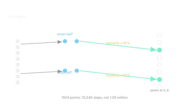
The FFT brackets frequencies the same way. Split samples into even and odd halves, transform each half (the sub-tournaments), then combine with twiddle-factor weights (the finals). Each of rounds costs combines: total instead of .
How It Actually Works
Radix-2 decimation in time: and , where are the half-size DFTs of even and odd samples. One butterfly computes both outputs from with one multiply. Recurse to size ; total operations. Bit-reversal permutes inputs so the recursion runs in place.
Bin means frequency for sampling rate ; resolution . Off-bin tones leak across bins; windowing (Hann: taper edges) localizes leakage at the cost of wider peaks.
Worked example
audio samples at Hz. Naive DFT: million complex multiplies. FFT: : ratio above . Resolution Hz per bin: a -Hz tone lands in bin exactly (), peak height amplitude. A -Hz tone straddles bins and (leakage): Hann windowing concentrates of its energy into bins instead of smearing over .
Code
import cmath
def fft(xs: list[complex]) -> list[complex]: n = len(xs) if n == 1: return xs # base case even = fft(xs[0::2]) odd = fft(xs[1::2]) # halve: decimation in time out: list[complex] = [0j] * n for k in range(n // 2): tw = cmath.exp(-2j * cmath.pi * k / n) * odd[k] # twiddle combine out[k] = even[k] + tw # butterfly top out[k + n // 2] = even[k] - tw # butterfly bottom return out
xs = [1.0, 0.0, -1.0, 0.0, 1.0, 0.0, -1.0, 0.0] # cosine, period 4spec = [round(abs(c), 3) for c in fft([complex(x) for x in xs])]print(spec) # -> peaks 4.0 at bins 2 and 6, zeros elsewhereBins and read (half the samples times amplitude ); all others : exact binning for an on-grid tone.
Watch Out For
Reading leaked bins as separate tones
One off-grid tone paints a skirt across many bins; peak-pickers report five tones where one exists. Window first, then interpolate the true peak (parabolic or Quinn estimators) instead of counting local maxima.
Zero-padding to fake resolution
Appending zeros interpolates the spectrum (smoother curve) without adding information: two tones Hz apart at -Hz resolution stay merged no matter the padding. Resolution comes from longer observation (), never from padding length.
The Quick Version
- The DFT bins finite samples; naive cost is .
- The FFT halves recursively through butterflies to .
- At the FFT needs steps versus million: times faster.
- Bin means Hz; resolution is ( Hz in the example).
- Off-grid tones leak; Hann windows concentrate energy threefold.
- Zero-padding smooths without resolving; longer records resolve.