Double and Triple Integrals

A single integral adds up along a line. Double and triple integrals add up over areas and volumes, which is how probabilities and masses get computed.

Four columns of heights 1.25, 1.75, 3.25 and 3.75 stand on the unit-by-two rectangle, and their volumes add to the integral value 5

Why Does This Exist?

Single integrals measure totals along a line: distance from speed, area under a curve. But ML quantities live over regions. A joint probability is an integral over a rectangle of outcomes. A mass is an integral over a volume. An expectation over two variables is an integral over their whole plane. None of these fit on a line, so the one-variable machinery from integration and area needs an upgrade that sums over areas and volumes instead.

Double and triple integrals are that upgrade, and their working method is reassuringly ordinary: integrate one variable at a time, turning a volume problem into a sequence of line problems. The same iteration pattern computes the normalizing constants behind integrals in probability.

The one idea you need first

A definite integral adds up infinitely many infinitesimal slices: $\int_a^b f(x)\, dx$ is the signed area under the curve. A double integral $\iint_R f(x, y)\, dA$ does the same over a region $R$ , stacking slices in two directions to get a volume. Add a third variable and the volume becomes a hypervolume, which sounds exotic but computes identically.

Think of It Like This

Counting grain in a silo with a grid of tubes

You need the grain volume in a rectangular silo with an uneven surface. Drop a grid of measuring tubes: each tube reads the depth at its spot, and depth times the tube's footprint is its share of the volume. Add every tube and you have the total.

A double integral is that procedure with the grid refined forever. Each point contributes height times infinitesimal footprint, and the integral is the sum. Iterated integration reads the silo one row of tubes at a time: finish a row (inner integral), then add the rows (outer integral). The order of rows versus columns never changes the grain total, which is the everyday content of Fubini's theorem.

The analogy stops at uniformity. Grain has constant density, but integrands vary, and probability densities must additionally total exactly one, which constrains the surface in ways grain never faces.

How It Actually Works

A double integral over a rectangle iterates: hold $y$ fixed and integrate over $x$ , then integrate the result over $y$ :

\iint_R f(x, y)\, dA = \int_{c}^{d}\left(\int_{a}^{b} f(x, y)\, dx\right) dy

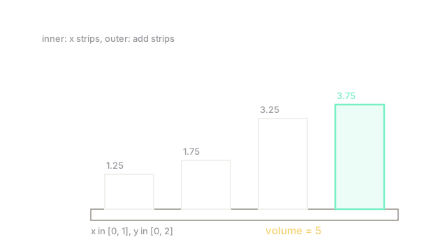
In plain words: the inner integral collapses each vertical strip to a number depending on $y$ , and the outer integral adds those strip totals. Fubini's theorem says that for continuous functions on rectangles, either order gives the same answer, so integrate in whichever order is easier. A triple integral adds one more nesting for volumes in three variables.

Two habits keep the computation honest. First, inner limits may depend on the outer variable when the region is not a rectangle, as with triangles or disks. Second, the differential carries the geometry: $dx\, dy$ for Cartesian grids, $r\, dr\, d\theta$ for polar ones, where the extra $r$ accounts for wedges widening outward.

Worked example

Integrate $f(x, y) = x + 2y$ over the rectangle $x \in [0, 1]$ , $y \in [0, 2]$ .

Inner integral over $x$ , treating $y$ as a constant: $\int_0^1 (x + 2y)\, dx = 1/2 + 2y$ . Outer integral over $y$ : $\int_0^2 (1/2 + 2y)\, dy = 1 + 4 = 5$ . So the volume under this tilted plane over the rectangle is exactly $5$ .

Reverse the order as a check: $\int_0^1\left(\int_0^2 (x + 2y)\, dy\right) dx = \int_0^1 (2x + 4)\, dx = 1 + 4 = 5$ . Same answer, as Fubini promises. For a triple taste: $\iiint_{[0,1]^3} (x + y + z)\, dV = 1/2 + 1/2 + 1/2 = 3/2$ , since each variable contributes its average $1/2$ over the unit cube.

Code

A midpoint Riemann sum with live code, converging to the hand-computed 5. Linear integrands converge fast: even a 4-by-4 grid is already exact.

1def midpoint(n: int) -> float:2    total = 0.03    for i in range(n):4        for j in range(n):5            x = (i + 0.5) / n        # x in [0, 1]6            y = 2 * (j + 0.5) / n    # y in [0, 2]7            total += x + 2 * y8    return total * (1 / n) * (2 / n)9
10
11print(midpoint(4))            # -> 5.012print(round(midpoint(50), 6))  # -> 5.0

Both print 5, matching the iterated hand calculation. The coarse grid is exact here only because the integrand is linear; curved surfaces need the fine grid to converge.

Watch Out For

Integrating in the convenient order over the wrong limits

Fubini lets you swap the order, but the limits must describe the same region after the swap. On a triangle like $0 \leq x \leq y \leq 1$ , integrating $x$ first needs $x$ from $0$ to $y$ , and swapping means $y$ from $x$ to $1$ . Copying rectangular limits onto a triangular region integrates over a square instead, doubling the answer's territory. Sketch the region before choosing limits.

Dropping the Jacobian in curved coordinates

Switching to polar or spherical coordinates without the $r$ or $r^2 \sin\phi$ factor integrates the right function over the wrong geometry, underweighting everything far from the origin. The factor is not decoration: it is the area of an infinitesimal wedge. Whenever coordinates curve, multiply by the Jacobian determinant.

The Quick Version

Double integrals sum over areas and triple integrals over volumes by iterating one variable at a time.
The inner integral collapses strips to numbers; the outer integral adds the strips.
Fubini says the order does not matter for continuous functions, so pick the easier order.
Non-rectangular regions need limits that depend on the outer variable; sketch first.
Curved coordinates need the Jacobian factor, or distant regions get underweighted.