Expectation-Maximization

Learning with missing labels by alternating guesses. Fill in the hidden assignments softly, refit the model, and repeat until neither moves.

Soft assignments pull two cluster means from their 0 and 3 starts to 0.3 and 4.1 in a single EM pass

Why Does This Exist?

Many models have hidden assignments: which Gaussian produced each point, which topic wrote each word, which state a tracker was in. Maximum likelihood wants complete data, but the labels are missing. Expectation-Maximization fills them in softly (as probabilities, not hard calls), refits the model to the filled-in data, and repeats. Likelihood rises every round, which makes EM one of the few iterative algorithms with a built-in progress certificate.

EM is the parent of a large family: k-means is its hard-assignment limit, Baum-Welch for hidden Markov models is EM on sequences, and variational inference generalizes its lower bound. This page teaches the core loop; mixtures and sequences get their own pages.

The one idea you need first

Maximum likelihood picks parameters maximizing $p(\text{data} \mid \theta)$ . With hidden $z$ , the likelihood $\sum_z p(x, z \mid \theta)$ has the sum inside the log, which blocks closed forms. EM instead maximizes a lower bound built from a guess at $z$ , tightens the guess, and repeats. The MLE background is in maximum likelihood estimation.

Think of It Like This

Two overlapping piles of exam papers

Two classes took the same exam and the piles got mixed. You must recover each class's average. Start with a guess (class A averages 0, class B averages 6). For each paper, estimate the probability it belongs to A versus B from the current averages (E step, soft sorting). Then recompute each average weighting papers by those probabilities (M step). Repeat.

Hard sorting (each paper wholly to one class) is k-means and it jitter. Soft sorting is EM: a borderline paper counts 60 percent toward A and 40 percent toward B, so one ambiguous paper cannot yank an average across the room. The averages and the sortings chase each other to a agreement neither could reach alone.

Where the analogy stops: real EM also refits variances and mixing weights each round, and the likelihood guarantee needs the exact posterior over assignments, not an approximation.

How It Actually Works

Parameters $\theta$ , observed $x$ , hidden $z$ . The E step computes responsibilities $\gamma(z) = p(z \mid x, \theta^{\text{old}})$ . The M step maximizes the expected complete log-likelihood:

\theta^{\text{new}} = \arg\max_\theta \sum_z \gamma(z) \log p(x, z \mid \theta)

Each round tightens a lower bound on $\log p(x \mid \theta)$ (E step) then climbs it (M step), so likelihood never decreases. EM converges to a local optimum, not necessarily the global one: starts matter.

Worked example

Four 1-D points $[0, 2, 4, 6]$ , two unit-variance Gaussians with equal weights, means started at $\mu_A = 0$ , $\mu_B = 6$ . E step: responsibility of A for $x$ is proportional to $\exp(-(x-\mu_A)^2/2)$ versus B's $\exp(-(x-\mu_B)^2/2)$ .

$x = 0$ : A unnormalized $1.0$ , B $\exp(-18) \approx 0$ . $\gamma_A \approx 1.0$ .
$x = 2$ : A $\exp(-2) \approx 0.135$ , B $\exp(-8) \approx 0.0003$ . $\gamma_A \approx 0.998$ .
$x = 4$ : A $\exp(-8) \approx 0.0003$ , B $\exp(-2) \approx 0.135$ . $\gamma_A \approx 0.002$ .
$x = 6$ : A $\approx 0$ , B $1.0$ . $\gamma_A \approx 0.0$ .

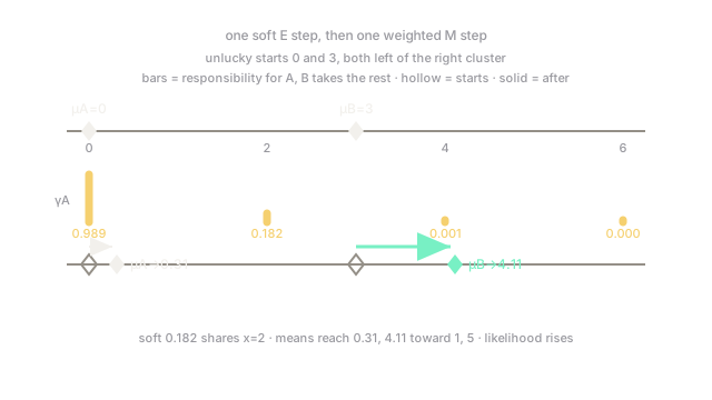
M step: $\mu_A = (1.0 \times 0 + 0.998 \times 2 + 0.002 \times 4 + 0 \times 6)/(1.0 + 0.998 + 0.002 + 0) = 2.004/2.0 \approx 1.0$ . Symmetrically $\mu_B \approx 5.0$ . Hmm, that barely moved from a lucky start. Make the start unlucky instead: $\mu_A = 0$ , $\mu_B = 3$ (both left of the right cluster).

$x = 0$ : A $1.0$ , B $\exp(-4.5) \approx 0.011$ . $\gamma_A \approx 0.989$ .
$x = 2$ : A $0.135$ , B $\exp(-0.5) \approx 0.607$ . $\gamma_A \approx 0.182$ .
$x = 4$ : A $0.0003$ , B $\exp(-0.5) \approx 0.607$ . $\gamma_A \approx 0.001$ .
$x = 6$ : A $\approx 0$ , B $\exp(-4.5) \approx 0.011$ . $\gamma_A \approx 0.0$ .

M step: $\mu_A = (0.989 \times 0 + 0.182 \times 2 + 0.001 \times 4)/1.172 = 0.368/1.172 \approx 0.31$ . $\mu_B = (0.011 \times 0 + 0.818 \times 2 + 0.999 \times 4 + 1.0 \times 6)/2.828 = 11.632/2.828 \approx 4.11$ . One pass moved the means from $(0, 3)$ to $(0.31, 4.11)$ , reaching toward the true clusters near 1 and 5. Continue and they settle near $(1.0, 5.0)$ ; the soft 0.182 assignment of $x = 2$ is what lets B claim it without a hard fight.

Code

One EM pass on the four points from the unlucky start, matching the hand numbers.

1import numpy as np2
3x = np.array([0.0, 2.0, 4.0, 6.0])  # data4mu = np.array([0.0, 3.0])  # unlucky start5like = np.exp(-0.5 * (x[:, None] - mu[None, :]) ** 2)  # Gaussian likelihoods6resp = like / like.sum(axis=1, keepdims=True)  # E step: responsibilities7mu = (resp * x[:, None]).sum(axis=0) / resp.sum(axis=0)  # M step8print(np.round(resp[:, 0], 3))  # -> A responsibilities9print(np.round(mu, 2))  # -> [0.31 4.11]

Responsibilities print $[0.989, 0.182, 0.001, 0.0]$ and means $[0.31, 4.11]$ . Loop the last two lines twenty times and the means land near $[1.0, 5.0]$ with likelihood higher every round.

Watch Out For

Local optima from a single start

EM climbs to the nearest peak, and mixture likelihoods have plenty: one component hogging everything, two components splitting one cluster, a variance collapsing onto a single point (infinite likelihood, useless model). Never run once. Run from many starts (k-means++ seeding helps) and keep the highest-likelihood result; collapse variances with a small floor.

Hardening responsibilities too early

Rounding soft assignments to 0/1 inside the loop turns EM into k-means mid-flight: the likelihood guarantee dies and borderline points swing whole means. Keep responsibilities soft until convergence, then harden once for reporting if labels are needed.

The Quick Version

EM alternates soft assignment of hidden labels (E step) with refitting to them (M step).
Likelihood rises every round, converging to a local optimum.
From the unlucky start $(0, 3)$ , one pass moves the means to $(0.31, 4.11)$ , heading for $(1, 5)$ .
Soft 0.182 assignments let clusters share borderline points instead of fighting over them.
k-means is the hard-assignment limit; Baum-Welch is EM on sequences.
Run many starts, floor the variances, and never harden responsibilities mid-loop.