Belief Propagation

Exact marginals by passing notes along the graph. Each node summarizes what its side believes, and the product of incoming notes is the answer.

Messages sweep forward and back along a three-node chain so each node combines both sides into its exact marginal

Why Does This Exist?

Factor graphs factor the joint, but you still need the marginals: $p(x_i)$ for every variable, for decisions, imputation, and learning. Brute force sums $2^{n-1}$ terms per variable. Belief propagation (the sum-product algorithm) turns that exponential into two linear sweeps on a tree, and into a celebrated approximation on loopy graphs that decodes turbo codes and calibrates stereo vision.

The idea is embarrassingly local. A message from node $a$ to neighbor $b$ summarizes everything $a$ 's side of the graph believes about the shared variable. Each node multiplies its incoming messages with its local factor and forwards the result. When the graph is a tree, two passes (leaves to root, root to leaves) make every marginal exact.

The one idea you need first

A marginal sums out everything else: $p(x_i) = \sum_{x \setminus x_i} p(x)$ . On a chain $A \to B \to C$ this factors into a forward sum over $A$ and a use of $p(C \mid B)$ , which is exactly one message each way. The factorization background is in probabilistic graphical models.

Think of It Like This

A telephone line settling a bet

Three friends in a line bet on whether it rained uphill. Ana saw the sky, Ben saw the road, Cat saw the gutter. Ana whispers to Ben her summary (forward message); Cat whispers to Ben hers (backward message). Ben combines both whispers with his own eyes and now holds the exact group verdict without anyone shouting across the line.

Nobody needed the full picture, only a summary passed along. If the three sat in a circle instead, whispers would loop and echo: each round refines the guess (loopy propagation), usually converging, sometimes resonating into overconfidence.

Where the analogy stops: messages are full distributions, not verdicts, and the combination rule is multiply-then-sum, not vote.

How It Actually Works

On a factor graph, the message from variable $x$ to factor $f$ is the product of all other incoming messages:

m_{x \to f}(x) = \prod_{g \neq f} m_{g \to x}(x)

The message from factor $f$ to variable $x$ sums the factor over its other variables:

m_{f \to x}(x) = \sum_{x_f \setminus x} f(x_f) \prod_{y \neq x} m_{y \to f}(y)

The marginal is proportional to the variable's local evidence times all incoming messages: $p(x) \propto \prod_f m_{f \to x}(x)$ . Schedule: on a tree, send from leaves inward, then outward. On loopy graphs, iterate until messages stop changing (no exactness guarantee, but strong practice).

Worked example

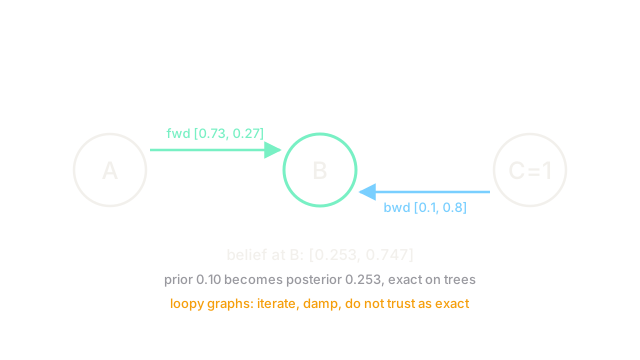
Reuse the alarm chain $A \to B \to C$ with $p(A{=}1) = 0.1$ , $p(B{=}1 \mid A{=}1) = 0.9$ , $p(B{=}1 \mid A{=}0) = 0.2$ , $p(C{=}1 \mid B{=}1) = 0.8$ , $p(C{=}1 \mid B{=}0) = 0.1$ , and observe $C = 1$ . Forward message $A \to B$ : $m(A{=}1) = 0.1$ , $m(A{=}0) = 0.9$ . Factor at $B$ combines: $m(B{=}1) = 0.9(0.1) + 0.2(0.9) = 0.27$ , $m(B{=}0) = 0.73$ . Backward message from the observation $C = 1$ : likelihood vector $[0.1, 0.8]$ over $B$ . Belief at $B$ : proportional to $[0.73 \times 0.1,\ 0.27 \times 0.8] = [0.073, 0.216]$ , normalized $[0.253, 0.747]$ . Backward to $A$ : $m(A{=}1) = 0.9(0.8) + 0.1(0.1) = 0.73$ times prior $0.1$ gives $0.073$ ; $m(A{=}0) = 0.2(0.8) + 0.8(0.1) = 0.24$ times $0.9$ gives $0.216$ . Normalized: $[0.747, 0.253]$ . Two passes, exact posterior $p(A{=}1 \mid C{=}1) = 0.253$ : the end belief moved from prior 0.10 to 0.25 on messages alone.

Code

Forward-backward on the chain, reproducing the hand computation.

1import numpy as np2
3pA = np.array([0.9, 0.1])4pB = np.array([[0.8, 0.2], [0.1, 0.9]])  # P(B|A), rows A5pC = np.array([[0.9, 0.1], [0.2, 0.8]])  # P(C|B), rows B6fwd = pA @ pB  # forward message at B: [0.73, 0.27]7bwd = pC[:, 1]  # backward message: likelihood of C=1: [0.1, 0.8]8post_B = fwd * bwd / (fwd * bwd).sum()9print(np.round(post_B, 3))  # -> [0.253 0.747]10mA = pB @ bwd * pA  # messages reach A, times prior11print(round(float(mA[1] / mA.sum()), 3))  # -> 0.253

Both prints give 0.253: the forward pass and the backward pass agree on the exact posterior. Replace the chain with a loop and rerun to feel loopy propagation converge (or oscillate) instead.

Watch Out For

Trusting loopy messages as exact

On trees the marginals are exact; on loopy graphs they are approximate and typically overconfident, because the same evidence cycles around and gets counted twice. People quote loopy beliefs with tree confidence and then wonder at miscalibration. Damp the updates (mix old and new messages) and validate against Gibbs samples on small cases before trusting a loopy deployment.

Underflow in long chains

Messages multiply many small numbers: a 1,000-node chain underflows float64 to zero and every marginal becomes NaN. Normalize messages at every step (only relative values matter) or work in log space. If your chain code works at length 50 and NaNs at 500, this is the cause, not the model.

The Quick Version

Belief propagation computes marginals by passing summary messages along graph edges.
Variable nodes multiply incoming messages; factor nodes multiply by the factor and sum out.
Two passes make tree marginals exact; iterating on loopy graphs is approximate but useful.
The worked chain moves the alarm belief from 0.10 to 0.253 with two passes.
Loopy beliefs run overconfident, so damp updates and cross-check with sampling.
Normalize every message or long chains underflow to NaN.