Mean-Field Approximation

Pretend every hidden variable decides on its own, ignoring the others, so a tangled joint posterior becomes a product of simple pieces you can update one at a time.

A coupled two-variable joint table is replaced by two independent Bernoulli factors, and one coordinate update moves the first factor to 0.71

Why Does This Exist?

Posteriors couple everything to everything. In a mixture model the cluster assignment of point 7 depends on the means, which depend on all the other assignments. In an Ising model each spin feels its neighbours. Exact inference sums over every joint configuration, and that sum has one term per combination: 2 hidden bits is 4 terms, 100 bits is about $10^{30}$ terms. Nobody sums that.

Expectation-maximization dodges the sum when the exact conditional over the hidden variables is available in closed form. Often it is not. Mean-field variational inference is the fallback with a guarantee: pick the closest distribution inside a tractable family, where closeness is KL divergence, and climb a lower bound instead of the true evidence. This page teaches the family and the coordinate climb. The bound itself is background in Bayesian inference.

The one idea you need first

For any distribution $q$ over hidden variables $z$ , $\log p(x) = \text{ELBO}(q) + \text{KL}(q \parallel p(z \mid x))$ . The ELBO is computable without the true posterior, and pushing it up pushes $q$ toward the posterior. Mean-field is the choice of which $q$ family to push inside.

Think of It Like This

A seating chart decided by independent ballots

A wedding planner must seat 100 guests with tangled friendships. The exact solution considers every seating at once. The mean-field planner does something humbler: each guest independently picks a table distribution, ignoring what any specific other guest does, and only responding to the average behaviour of the rest.

Round by round, guest 1 updates against the current averages of guests 2 through 100, then guest 2 updates, and so on. Nobody ever reasons about a joint seating. The plan converges to tables that are good on average, but it can never represent "Alice and Bob must sit together or both leave": that statement is about correlation, and independent ballots cannot say it.

Where the analogy stops: real mean-field factors are distributions with parameters, and the update is an exact expectation under the other factors, not a vote.

How It Actually Works

Write the hidden variables as $z = (z_1, \ldots, z_M)$ and restrict $q$ to factorize:

q(z) = \prod_{i=1}^{M} q_i(z_i)

In plain words: each hidden piece gets its own distribution, and the joint is their product. No correlations survive: under $q$ , learning $z_1$ tells you nothing about $z_2$ . That is the whole approximation, and everything good and bad about mean-field flows from it.

Holding all factors except $q_j$ fixed, the ELBO is maximized by

q_j(z_j) \propto \exp\!\left( \mathbb{E}_{q_{-j}}[\log p(x, z)] \right)

where $q_{-j}$ means all factors except $j$ . In plain words: set factor $j$ from the average log-joint, averaging over everyone else's current beliefs. Cycling $j = 1, \ldots, M$ is coordinate-ascent variational inference (CAVI). Each step raises the ELBO, so the procedure converges to a local optimum of the bound, exactly like EM converges to a local optimum of likelihood.

Worked example

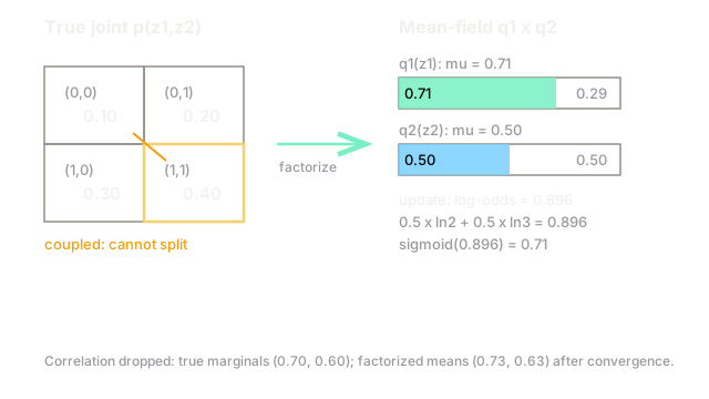
Two binary variables with joint table $p(0,0) = 0.10$ , $p(0,1) = 0.20$ , $p(1,0) = 0.30$ , $p(1,1) = 0.40$ . Use $q(z_1, z_2) = \text{Bernoulli}(\mu_1)\,\text{Bernoulli}(\mu_2)$ and start both at $0.50$ .

Fix $\mu_2 = 0.50$ and update factor 1. The log-odds under the optimal $q_1$ is the averaged log-ratio:

\log\frac{\mu_1}{1 - \mu_1} = \mu_2 \log\frac{0.40}{0.20} + (1 - \mu_2)\log\frac{0.30}{0.10}

Substituting $\mu_2 = 0.50$ : $0.50 \times 0.693 + 0.50 \times 1.099 = 0.896$ . So $\mu_1 = 1/(1 + e^{-0.896}) \approx 0.71$ .

One coordinate step moved the first factor from $0.50$ to $0.71$ , leaning toward 1 because three of the four table entries by mass favour $z_1 = 1$ . Continuing to alternate settles near $(0.73, 0.63)$ . The true marginals are $p(z_1 = 1) = 0.70$ and $p(z_2 = 1) = 0.60$ : close on means, while the true correlation between the variables is silently dropped, which is the next section's warning.

Watch Out For

Trusting the reported uncertainty

Mean-field posteriors are systematically overconfident. Because $q$ cannot represent correlation, it picks one mode and reports that mode's width as the whole uncertainty, exactly like variational inference under-reports in the Bayesian inference page. A mean-field logistic regression can report 99 percent confidence on weights whose true posterior spans a wide correlated ridge.

Symptom: decisions that need calibrated uncertainty (active learning, bandits, safety checks) fail while point predictions look fine. Fix: read only the means from mean-field, and get uncertainty from MCMC, a full-rank Gaussian, or at least a structured factorization that keeps the important correlations.

Strong coupling stalls or flips the coordinate updates

When variables are tightly coupled, updating one at a time crawls: each factor's optimum barely moves given the others, so CAVI takes tiny steps along a narrow valley. Worse, with symmetric multimodality (two equally good explanations), the initialization decides the mode and the updates never visit the other.

Symptom: different random starts land on qualitatively different factorizations with similar ELBOs. Fix: run several starts and keep the best bound, consider damping the updates, and if two variables are nearly locked together, merge them into one joint factor (structured mean-field) instead of factorizing across the lock.

The Quick Version

Mean-field replaces $p(z \mid x)$ with a product $q(z) = \prod_i q_i(z_i)$ , deleting all correlations by construction.
Each factor updates from the averaged log-joint under the other factors, and cycling them (CAVI) climbs the ELBO to a local optimum.
On the worked table, one update moves $\mu_1$ from 0.50 to 0.71, near the true marginal 0.70.
Means are usually decent; variances and correlations are not: expect overconfidence.
Strongly coupled variables need joint factors, multiple starts, or a richer family.