Moments and Moment Generating Functions

Why Does This Exist?

Full distributions are heavy objects: densities, tables, or samplers you must carry everywhere. Most decisions need only a few summaries. Where is the center, how wide is the spread, does it lean, how heavy are the tails? Moments answer exactly those four questions, in order, and entire fields run on the first two: portfolio theory is mean versus variance, and the central limit theorem says large sums forget everything but their first two moments.

Moment generating functions earn their place by making moments mechanical. Instead of integrating $x^k$ against the density separately for each $k$, differentiate one function at zero and read the answers off. They also prove distribution facts cleanly: sums of independent variables multiply MGFs, which is the two-line reason normals add to normals. The mean and variance groundwork is expectation, variance and covariance; the Fourier sibling that always exists is characteristic functions.

The one idea you need first

The $k$-th raw moment is $E[X^k]$: the average of the $k$-th power. The $k$-th central moment recenters first: $E[(X - \mu)^k]$. So the mean is the first raw moment, the variance is the second central moment, skewness standardizes the third, and kurtosis standardizes the fourth. Each moment sees one more shape of the distribution than the last.

Think of It Like This

How It Actually Works

The moment generating function is the expectation of the exponential tilt:

In plain words: weight each outcome by $e^{tx}$ and average. Differentiating under the expectation pulls down one $X$ per derivative, so $M_X^{(k)}(0) = E[X^k]$, the $k$-th raw moment. Mean from one derivative, second moment from two, variance from their combination $\text{Var}(X) = M''(0) - M'(0)^2$.

Three properties do the heavy lifting. First, sums of independent variables multiply MGFs: $M_{X+Y} = M_X M_Y$, which is why the normal family, the Poisson family, and the gamma family with shared rate all stay in the family under addition. Second, matching MGFs near zero identify the distribution, so proving convergence of MGFs proves convergence in distribution. Third, the log-MGF generates cumulants, where the normal keeps only two nonzero terms and every extra term measures non-Gaussianity.

Worked example

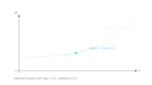
Take a Bernoulli with $p = 0.3$. Its MGF is $M(t) = 0.7 + 0.3e^t$: still 0 with chance 0.7, tilted by $e^t$ with chance 0.3.

First derivative: $M'(t) = 0.3e^t$, so $M'(0) = 0.3$, the mean. Second: $M''(t) = 0.3e^t$, so $M''(0) = 0.3$, the second moment. Variance is their combination: $0.3 - 0.3^2 = 0.3 - 0.09 = 0.21$. The diagram draws this MGF leaving $(0, 1)$ with slope $0.3$, and that slope is the mean made visible.

Code

Two derivatives of the Bernoulli MGF by finite differences, recovering the mean and variance without any integration.

1import math2
3p = 0.34
5
6def mgf(t: float) -> float:7    return (1 - p) + p * math.exp(t)  # Bernoulli MGF8
9
10h = 1e-511mean = (mgf(h) - mgf(-h)) / (2 * h)12second = (mgf(h) - 2 * mgf(0) + mgf(-h)) / h**213print(round(mean, 6))          # -> 0.314print(round(second - mean**2, 3))  # -> 0.21

The prints give 0.3 and 0.21, matching the hand derivation. Differentiation at zero replaced two expectation integrals, which is the whole point of the machine.

Watch Out For

The Quick Version

• Moments are shape summaries in order: center, spread, lean, tail weight.
• The MGF packs them into one function, with the k-th derivative at zero giving the k-th moment.
• MGFs multiply across independent sums, which is why some families stay closed under addition.
• Bernoulli 0.3 yields mean 0.3 and variance 0.21 from two derivatives.
• Heavy-tailed distributions may have no MGF, and moments alone never identify a distribution.

What to Read Next

• Expectation, Variance and Covariance
• Probability Distributions
• Characteristic Functions