Exploration-Exploitation Theory

Every learner must choose between cashing in on the best known action and testing rivals, and bandit theory prices that choice with regret bounds you can compute.

An optimistic rule keeps testing the uncertain arm until its confidence bound falls below the known good arm

Why Does This Exist?

Greedy learning fails quietly: pick the current best action forever and a slightly better action you tried once on a bad day stays buried. Pure exploration fails loudly, burning reward on known-bad choices. Production systems from ad ranking to clinical trials need a principled middle that wastes little while still discovering.

Bandit theory supplies it with regret: total reward lost versus always playing the best arm. It proves greedy suffers linear regret while optimism and Thompson sampling pay only logarithmic regret. This page defines regret and derives the UCB rule.

The one idea you need first

A confidence interval says the true mean lies within estimate plus or minus a width that shrinks as $1/\sqrt{n}$ with $n$ samples. Few samples mean wide intervals and real uncertainty. Confidence intervals carry the construction.

Think of It Like This

Choosing a lunch spot in a new town

Two cafes sit nearby. You have eaten at A five times (good, consistent) and at B once (bad day, maybe unfair). Greedy eats at A forever. A food critic friend says: score each place by its average plus a bonus for uncertainty, and visit the higher score. B's bonus keeps it alive for a second visit, and after a few tries its interval tightens and the contest ends honestly.

The bonus is the exploration term $\sqrt{\ln t / n}$ , and dropping it is pure greed. Where the analogy stops: cafe quality drifts with chefs, while basic bandit theory assumes fixed means, so drifting tastes need windowed variants.

How It Actually Works

With $K$ arms and horizon $T$ , regret is:

R_T = T \mu^* - \sum_{t=1}^T \mathbb{E}[\mu_{A_t}]

In plain words: $\mu^*$ is the best arm's mean, $A_t$ is the arm pulled at $t$ , and regret totals the gap. Logarithmic $R_T \sim \log T$ means per-step loss vanishes; linear means it never does.

UCB1 pulls the arm maximizing $\hat{\mu}_i + \sqrt{2 \ln t / n_i}$ : estimate plus uncertainty. Arms pulled rarely have large bonuses and get retried; well-sampled losers fall behind forever. Its regret is bounded by about $\sum_{bad} 8 \ln T / \Delta_i$ , where $\Delta_i$ is the arm's gap to best. Epsilon-greedy with fixed $\epsilon$ explores randomly a fraction $\epsilon$ of the time and pays linear regret $\sim \epsilon T \Delta$ .

Worked example

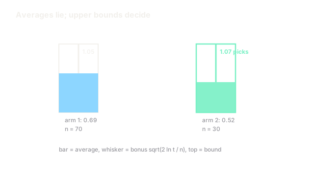
Two arms, means $0.7$ and $0.5$ , gap $\Delta = 0.2$ . At $t = 100$ , suppose arm 1 sampled 70 times averaging $0.69$ , arm 2 sampled 30 times averaging $0.52$ .

UCB bonuses with $\sqrt{2 \ln t / n}$ : arm 1 gets $\sqrt{2 \times 4.605/70} = \sqrt{0.1316} \approx 0.363$ , total $1.053$ . Arm 2 gets $\sqrt{2 \times 4.605/30} = \sqrt{0.307} \approx 0.554$ , total $1.074$ . UCB pulls arm 2 despite its lower average, correctly buying information. After arm 2 reaches 60 pulls with average $0.50$ , its bonus falls to $\sqrt{0.1535} \approx 0.392$ for $0.892$ versus arm 1 at $0.69 + 0.34 = 1.03$ , and exploitation resumes.

Code

1import numpy as np2
3
4def ucb_pick(means: np.ndarray, counts: np.ndarray, t: int) -> int:5    bonus = np.sqrt(2 * np.log(t) / np.maximum(counts, 1))  # wide when untried6    return int(np.argmax(means + bonus))  # optimism wins7
8
9means = np.array([0.69, 0.52])10counts = np.array([70, 30])11print(ucb_pick(means, counts, 100))  # -> 1

Index 1 is the second arm, matching the hand totals 1.053 versus 1.074. The bonus term is doing the exploration arithmetic.

Watch Out For

Fixed epsilon that never decays

Epsilon-greedy with $\epsilon = 0.1$ keeps pulling random arms 10 percent of the time forever, paying linear regret around $0.1 T \Delta$ . On a year of traffic that is a permanent tax. The symptom is a learning curve that improves then flatlines below UCB.

Decay $\epsilon$ like $1/t$ or switch to UCB or Thompson sampling for long horizons.

Applying stationary bounds to drifting arms

UCB1's logarithm assumes fixed means. When rewards drift (weekend traffic differs), old samples mislead and the bound breaks: the algorithm trusts stale winners. Regret turns linear again with no warning in the logs.

Use sliding windows or discounted UCB when the world moves, and monitor per-arm means over time.

The Quick Version

Regret totals reward lost versus the best arm; logarithmic regret means learning, linear means stuck.
UCB adds $\sqrt{2 \ln t / n}$ to each average and pulls the max, earning logarithmic regret.
The $0.7$ versus $0.5$ example pulls the worse-looking arm at 30 samples and stops at 60.
Fixed epsilon-greedy pays a permanent linear tax; decay it or use optimism.
Stationary rules fail on drifting rewards, so window the history when the world moves.