Graph Laplacian

Degree minus adjacency: the matrix that turns "neighbours should agree" into arithmetic, so connectivity becomes eigenvalues you can compute.

A triangle graph with degree 2 on every diagonal and minus 1 on every edge gives a Laplacian whose quadratic form counts 6 units of disagreement

Why Does This Exist?

Graph fundamentals turned edges into an adjacency matrix and showed powers count walks. But adjacency answers "how do I get there", not "how tightly does this hold together" or "what assignment varies least across edges". Those need a matrix whose energy measures disagreement. The Laplacian is that matrix, and it is the object behind spectral clustering, Laplacian smoothing in graph networks, and semi-supervised label spreading. The spectral consequences (Fiedler cuts, normalized variants, smoothing dynamics) get their full treatment in spectral views; this page builds the object itself.

The one idea you need first

For degrees $D$ (diagonal) and adjacency $A$ , $L = D - A$ has each degree on its diagonal and $-1$ per edge, so every row sums to zero and the constant vector is always in its null space. That zero row sum is the source of every theorem below.

Think of It Like This

Tension in a net of ropes

Knot a rope net: each knot's tension equals how far it sits from the average of its tied neighbours, times its number of ties. A knot dead-centered among its neighbours feels nothing; a knot dragged away from them feels pull proportional to the disagreement.

The Laplacian computes exactly that tension pattern for any assignment of positions to knots. Assignments where neighbours agree have low total tension; the all-equal assignment has zero. Spectral methods then ask which non-flat assignment has the least tension, and that answer cuts the net where it is weakest.

Where the analogy stops: ropes pull in physical space, while the Laplacian acts on any signal (labels, features, voltages) living on the nodes.

How It Actually Works

For $n$ nodes with adjacency $A$ and degree matrix $D_{ii} = \deg(i)$ :

L = D - A

In plain words: diagonal holds degrees, off-diagonal holds $-1$ per edge (or minus the weight for weighted graphs). $L$ is symmetric for undirected graphs, positive semi-definite, with smallest eigenvalue $0$ on the all-ones vector.

The disagreement identity

For any signal $x$ assigning one number per node:

x^\top L x = \sum_{(i,j) \in E} (x_i - x_j)^2

Each edge contributes the squared gap across it. Consequences: $x^\top Lx \ge 0$ always (positive semi-definite); it is zero exactly when $x$ is constant on each component; minimizing it asks for the smoothest non-constant signal, which is why it regularizes semi-supervised learning and why message passing smooths.

Worked example

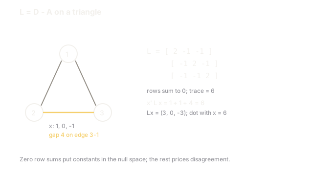
Triangle $1 - 2 - 3 - 1$ . Every degree is $2$ :

L = \begin{bmatrix} 2 & -1 & -1 \\ -1 & 2 & -1 \\ -1 & -1 & 2 \end{bmatrix}

Row sums: $2 - 1 - 1 = 0$ on every row, confirming the constant vector maps to zero. Trace is $6$ .

Take signal $x = (1, 0, -1)$ . Edge gaps: $(1-0)^2 = 1$ , $(0-(-1))^2 = 1$ , $((-1)-1)^2 = 4$ . Sum: $1 + 1 + 4 = 6$ . By matrix: $Lx = (3, 0, -3)^\top$ (check row 1: $2(1) - 0 - (-1) = 3$ ), then $x^\top Lx = 1(3) + 0(0) + (-1)(-3) = 6$ . Both routes agree. The signal disagrees most across edge $(3,1)$ , and the quadratic form prices exactly that.

Watch Out For

Using the unnormalized Laplacian on heavy-tailed graphs

Minimizing $x^\top Lx$ minimizes raw cut edges with no penalty for tiny pieces, so on social or citation graphs the optimal cut lops off one low-degree node. You asked for two communities and got a singleton plus everything else.

Symptom: recursive bisection peels singletons repeatedly. Fix: normalize by volume ( $L_{\mathrm{sym}}$ or random-walk), which divides cut size by cluster volume, as the spectral views page details.

Testing zero eigenvalues with exact equality

The zero eigenvalue returns as $-3 \times 10^{-16}$ , and exact $== 0$ tests then report a connected graph as disconnected or miss components. Never let a tiny negative value flow into a square root either.

Symptom: component counts flicker between runs, or nan appears from sqrt of a small negative. Fix: count with vals < 1e-8 and clamp negatives to zero before roots.

The Quick Version

$L = D - A$ : degrees on the diagonal, minus 1 per edge, zero row sums.
$x^\top Lx$ sums squared gaps across edges, so it measures disagreement.
$L$ is symmetric positive semi-definite with eigenvalue 0 on constants.
On the triangle, signal $(1, 0, -1)$ scores exactly 6 by edges and by matrix.
Zero eigenvalue multiplicity counts components; the rest measures cohesion.
Normalize on uneven graphs, and never test floating eigenvalues for exact zero.