Math

Graph Laplacian and Spectral Views

Degree minus adjacency turns a graph into a matrix whose eigenvalues describe how connected it is — which is how a discrete structure becomes something linear algebra can answer questions about.

The Laplacian of a four-node path has eigenvalues 0, 0.586, 2 and 3.414, and the eigenvector for 0.586 changes sign exactly across the middle edge — which is where the graph is weakest and where a two-way cut belongs

Why Does This Exist?

Because a graph is not a matrix, and everything in linear algebra needs one.

You have eigenvalues, decompositions, projections and least squares — a large toolkit that operates on matrices. A graph is a set of nodes and a set of edges: no rows, no columns, nothing to decompose. Graph fundamentals already made the first move, the adjacency matrix, and showed that matrix powers count walks. This page makes the second and more consequential one.

The Laplacian is the matrix that makes spectral methods work, and it earns its place because its eigenvalues answer questions about the graph that are otherwise combinatorial and expensive:

Is the graph connected, and how strongly? The count of zero eigenvalues is exactly the number of connected components — a global structural fact read off a spectrum. The smallest non-zero eigenvalue measures how close the graph is to falling apart.
Where should it be cut in two? Finding a minimum balanced cut is NP-hard. The eigenvector of the second-smallest eigenvalue gives a good one in polynomial time, and that is spectral clustering in one sentence.
What does a graph neural network actually compute? A GCN layer is $\hat{A} H W$ where $\hat{A}$ is a normalised adjacency with self-loops — which is $I$ minus a normalised Laplacian. Every message-passing layer is a step of Laplacian smoothing, and once you see that, over-smoothing stops being a mystery and becomes a prediction.
How do you embed a graph in continuous space? Laplacian eigenmaps, and by extension the manifold-learning family that includes spectral embedding and diffusion maps, use the low eigenvectors as coordinates.

There is a fifth payoff worth naming: this is where eigenvalues pay off a second time, on an object that is not obviously geometric. The first payoff was PCA on a covariance matrix. This one says something about connectivity, which is a much less expected place for a spectrum to be informative.

Think of It Like This

A network of springs, and where it pulls apart

Imagine each node of the graph is a bead and each edge is a spring of equal stiffness. Beads not joined by an edge exert no force on each other.

Now pull the whole assembly apart and let it settle into its natural modes of vibration, the way a guitar string settles into a fundamental and its harmonics. Each mode is a pattern of displacement, and each has a frequency.

The lowest mode is trivial: every bead moves together, in the same direction, by the same amount. No spring stretches, so the frequency is zero. This is the constant eigenvector, and it carries no information — it exists for every graph and is the thing you always discard.

The second-lowest mode is the informative one. Something has to actually stretch, and the springs will arrange it so that the fewest and weakest connections do the stretching. Half the assembly moves one way, half the other, and the boundary between them falls wherever the structure is thinnest. That eigenvector is the Fiedler vector, and its sign pattern is a good cut of the graph. Its frequency, the algebraic connectivity, says how hard the assembly resists being pulled apart at all.

Two consequences fall straight out of the picture:

If the assembly is in two separate pieces, there are two zero-frequency modes — each piece can drift on its own without stretching anything. Three pieces, three zero modes. The multiplicity of eigenvalue zero counts the components, and this is not a coincidence to memorise but a fact you can see.

A weakly-attached single bead is also cheap to move. Hang one bead off the assembly by a single spring and the second mode may simply be that bead moving on its own — a technically correct answer to "what is easiest to separate" and a useless answer to "how do I split this into two groups". This is exactly the failure that the normalised Laplacian fixes, and it is the first pitfall.

How It Actually Works

The definition is a subtraction:

L = D - A

where $A$ is the adjacency matrix and $D$ is the diagonal matrix of degrees, $D_{ii} = \deg(i)$ . So $L$ has each node's degree on its diagonal and $-1$ wherever an edge exists. Every row sums to zero, which is the whole reason the constant vector is in the null space.

The identity that explains everything

For any vector $x$ assigning a number to each node:

x^\top L x = \sum_{(i,j) \in E} (x_i - x_j)^2

In plain words: the Laplacian quadratic form is the total squared disagreement across edges. That is the most useful single line on this page, and three things follow from it immediately.

$L$ is positive semi-definite. The right-hand side is a sum of squares, so it is never negative. Every eigenvalue is therefore $\ge 0$ , which is what makes the positive-definite machinery apply.

$x^\top L x = 0$ exactly when $x$ is constant on each connected component. No edge can join two nodes with different values, so within a component every value must be equal. This is the theorem about zero eigenvalues, proved in one step.

Minimising $x^\top L x$ is asking for a smooth signal on the graph. Neighbours should agree. This is the regularisation term in semi-supervised learning on graphs, the smoothness prior in graph signal processing, and precisely what a message-passing layer moves a representation toward.

The spectrum and what to read from it

Sort the eigenvalues $0 = \lambda_1 \le \lambda_2 \le \cdots \le \lambda_n$ .

$\lambda_1 = 0$ always, with the all-ones eigenvector. Free, and uninformative.
The number of zero eigenvalues is the number of connected components.
$\lambda_2$ is the algebraic connectivity — the Fiedler value. Zero means disconnected; small means there is a near-bottleneck; large means well-knit. It bounds the sparsest cut from both sides via Cheeger's inequality, which is what makes spectral clustering a method with a guarantee rather than a heuristic.
The corresponding eigenvector is the Fiedler vector. Threshold it at zero and you have a cut.
$\lambda_n \le 2\max_i \deg(i)$ , so the spectrum's top end is bounded by the densest node.

Normalising it, and why GNNs are Laplacian smoothing

The unnormalised $L$ weights high-degree nodes more heavily, simply because their diagonal entries are larger. Two standard normalisations remove that:

L_{\mathrm{sym}} = D^{-1/2} L D^{-1/2} = I - D^{-1/2} A D^{-1/2}, \qquad L_{\mathrm{rw}} = D^{-1} L = I - D^{-1}A

$L_{\mathrm{sym}}$ is symmetric with eigenvalues in $[0, 2]$ ; $L_{\mathrm{rw}}$ is the random-walk version. Normalised cuts (NCut) uses $L_{\mathrm{sym}}$ and is the default for clustering, because it optimises cut size relative to cluster volume and therefore prefers balanced partitions.

Now look at a GCN layer:

H^{(\ell+1)} = \sigma\!\left( \tilde{D}^{-1/2}\tilde{A}\,\tilde{D}^{-1/2} H^{(\ell)} W^{(\ell)} \right), \qquad \tilde{A} = A + I

The propagation matrix $\tilde{D}^{-1/2}\tilde{A}\tilde{D}^{-1/2}$ is exactly $I - L_{\mathrm{sym}}$ on the self-looped graph. So each layer replaces every node's features with a degree-weighted average over its neighbourhood — one step of diffusion. That is the whole architecture, and the self-loop is there to shift the spectrum away from the $\lambda = 2$ end where repeated application would oscillate rather than smooth.

The prediction this makes is testable and correct: stack enough layers and every node converges to the same representation. Repeated multiplication by a matrix drives any vector toward its dominant eigenvector, and here that is the smooth constant one. This is over-smoothing, it is why plain GCNs peak at 2 or 3 layers, and it is not a training difficulty — it is the fixed point of the operator you chose. Residual connections, PairNorm and initial-residual designs like GCNII all exist to fight this specific eigenvector.

Worked example

A path of four nodes: $1 - 2 - 3 - 4$ . Degrees are $1, 2, 2, 1$ .

L = D - A = \begin{bmatrix} 1 & -1 & 0 & 0 \\ -1 & 2 & -1 & 0 \\ 0 & -1 & 2 & -1 \\ 0 & 0 & -1 & 1 \end{bmatrix}

Every row sums to zero, so $L\mathbf{1} = \mathbf{0}$ and the all-ones vector is confirmed as an eigenvector for $\lambda = 0$ before computing anything.

The path graph has a closed form, $\lambda_k = 2 - 2\cos(k\pi/n)$ for $k = 0, \ldots, n-1$ :

\lambda = \{\,0,\ \ 2 - \sqrt{2} = 0.5858,\ \ 2,\ \ 2 + \sqrt{2} = 3.4142\,\}

Check the trace, which must equal the sum of eigenvalues and also the sum of degrees:

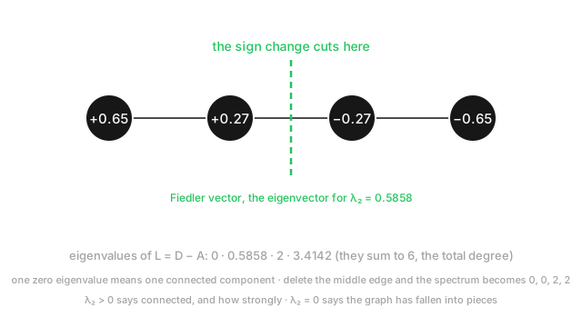
\mathrm{tr}(L) = 1 + 2 + 2 + 1 = 6, \qquad 0 + 0.5858 + 2 + 3.4142 = 6 \ \checkmark

One zero eigenvalue, so one connected component. Correct — a path is connected. And $\lambda_2 = 0.5858$ , comfortably above zero but well below the maximum degree, which is the signature of a chain: connected, but with an obvious weak point.

The Fiedler vector, normalised, is

v_2 = (0.6533,\ 0.2706,\ -0.2706,\ -0.6533)

Verify one entry by hand. Row 1 of $Lv_2$ is $1(0.6533) - 1(0.2706) = 0.3827$ , and $\lambda_2 v_{2,1} = 0.5858 \times 0.6533 = 0.3827$ . It checks.

Now read the signs: $(+, +, -, -)$ . The sign change falls between nodes 2 and 3 — the middle edge, which is exactly where a path should be cut in half. The eigenvector found the right answer with no combinatorial search. Notice also that the magnitudes decrease toward the centre, so the entries nearest the cut are the ones the method is least confident about.

Finally, delete that middle edge, leaving two disjoint edges $1-2$ and $3-4$ . The Laplacian becomes two blocks of $\begin{bmatrix} 1 & -1 \\ -1 & 1\end{bmatrix}$ , whose eigenvalues are $0$ and $2$ , so the full spectrum is

\lambda = \{\,0,\ 0,\ 2,\ 2\,\}

Two zero eigenvalues, two components. The algebraic connectivity dropped from 0.5858 to exactly 0, which is what "the graph fell apart" looks like in a spectrum.

Show Me the Code

1import numpy as np2
3A = np.array([[0, 1, 0, 0], [1, 0, 1, 0],       # path 1-2-3-4, shape (4, 4)4              [0, 1, 0, 1], [0, 0, 1, 0]], dtype=float)5L = np.diag(A.sum(1)) - A                        # degree minus adjacency6vals, vecs = np.linalg.eigh(L)                   # eigh: L is symmetric PSD7print(np.round(vals, 4))                         # -> [-0. 0.5858 2. 3.4142]8print(round(float(vals.sum()), 4), float(np.trace(L)))   # -> 6.0 6.09
10fiedler = vecs[:, 1]                             # skip column 0, the constant vector11print(np.round(fiedler * np.sign(fiedler[0]), 4))  # -> [0.6533 0.2706 -0.2706 -0.6533]12print(np.sign(fiedler * np.sign(fiedler[0])))      # -> [1. 1. -1. -1.]  cut the middle edge13
14x = np.array([1.0, 1.0, -1.0, -1.0])             # the quadratic form counts disagreement15print(float(x @ L @ x))                          # -> 4.0 == (1-(-1))^2 across one edge16
17A[1, 2] = A[2, 1] = 0.0                          # delete the middle edge18L2 = np.diag(A.sum(1)) - A19print(np.round(np.linalg.eigvalsh(L2), 4))       # -> [0. 0. 2. 2.]  two components

Every printed value matches the hand calculation. Two details in the output are worth noticing rather than skipping past.

The first eigenvalue prints as -0., not 0. — the true value is exactly zero and floating-point arithmetic delivered a tiny negative number that rounding rendered as negative zero. This is why the multiplicity of zero is tested with vals < 1e-8 and never with == 0, and why feeding an eigenvalue into a sqrt without clamping produces nan on a mathematically valid graph.

The np.sign(fiedler[0]) factor is not cosmetic either. An eigenvector's sign is arbitrary, so code that reads a partition from one must fix the orientation, or the two clusters swap labels between runs on identical input.

Watch Out For

Taking the smallest eigenvector, or reading a partition from an unoriented one

Three sign-and-index traps sit on top of each other here, and each produces a result that looks plausible.

The smallest eigenvector is the constant one. np.linalg.eigh returns eigenvalues ascending, so column 0 is the all-ones vector, always, for every connected graph. Threshold it and you get a partition determined entirely by floating-point noise around a constant — which produces a different, arbitrary split on every run and on every machine. You want column 1, and for a $k$ -way clustering you want columns 1 through $k-1$ . Off-by-one here is the most common bug in a hand-rolled spectral clustering.

On a disconnected graph there are several zero eigenvalues, so "column 1" is no longer the Fiedler vector. Check the multiplicity of zero first — np.sum(vals < 1e-8) — and if it exceeds 1 the graph is already partitioned and spectral clustering is answering a question you did not ask. Run a connected-components pass first.

Eigenvector signs are arbitrary. If $v$ is an eigenvector then so is $-v$ , and LAPACK makes no promise about which you get. Cluster labels will therefore flip between runs on identical input, which breaks any cached mapping from cluster ID to meaning and makes results look non-deterministic when they are not. Fix the orientation explicitly, as the code does.

And repeated eigenvalues have no unique eigenvector at all. A symmetric graph — a cycle, a complete bipartite graph, a regular lattice — has genuinely repeated eigenvalues, and any rotation within that eigenspace is an equally valid answer. The returned basis is then an arbitrary choice, and a partition read from it is arbitrary too. Check the gap $\lambda_3 - \lambda_2$ : if it is near zero, the spectral cut is not well defined and no amount of care in the code will make it stable.

Using the unnormalised Laplacian on a graph with uneven degrees, or a dense one at scale

Two separate ways this goes wrong in practice: the wrong matrix, and a matrix too large to hold.

The wrong matrix. Minimising $x^\top L x$ with the unnormalised Laplacian minimises the number of edges cut, with no reference to how big the resulting pieces are. On a real graph with a heavy-tailed degree distribution — which is nearly every social, citation or web graph — the cheapest cut is to lop off a single low-degree node. You asked for two clusters and got one node and everything else, repeatedly, at every level of a recursive bisection.

The fix is to normalise by volume, which is what NCut and $L_{\mathrm{sym}}$ do: the objective becomes cut size divided by cluster volume, so tiny clusters are penalised. Use the normalised Laplacian by default and treat unnormalised as the special case for near-regular graphs. In scikit-learn this is SpectralClustering(affinity=..., assign_labels='kmeans'), which uses the normalised version; and note the further detail that for $k > 2$ you row-normalise the eigenvector matrix before k-means, which is the step that makes multi-way spectral clustering work rather than merely run.

A matrix too large. A dense Laplacian for $n$ nodes is $n^2$ floats: one million nodes is 4 TB in float32 and a full eigh is $O(n^3)$ , which is not a long wait but an impossible one. Real graphs are sparse — average degree in the tens — so:

Store the Laplacian sparse. scipy.sparse CSR, built from the edge list, never materialising the dense form. Memory becomes $O(|E|)$ .
Ask only for the few eigenvectors you need. scipy.sparse.linalg.eigsh(L, k=8, sigma=0, which='LM') uses a shift-invert Lanczos iteration and touches the matrix only through matrix–vector products. Never call eigsh with which='SM' on a Laplacian — convergence to the smallest eigenvalues is notoriously slow, and shift-invert around zero is the standard remedy.
Consider LOBPCG or a multilevel method at tens of millions of nodes, where even Lanczos struggles. Or drop spectral methods and use Louvain or Leiden modularity clustering, which are near-linear and often good enough.
Watch for numerical drift in the zero eigenvalue. It should be exactly 0 and will come back as something like $-3 \times 10^{-16}$ . Never test == 0, and never let a tiny negative value propagate into a $\sqrt{\lambda}$ .

The Quick Version

The Laplacian is $L = D - A$ : degree on the diagonal, $-1$ per edge, every row summing to zero.
$x^\top L x = \sum_{(i,j) \in E} (x_i - x_j)^2$ . This one identity proves $L$ is positive semi-definite and explains what its eigenvectors mean.
Eigenvalue 0 always exists with the all-ones eigenvector. Its multiplicity is the number of connected components.
$\lambda_2$ is the algebraic connectivity: zero means disconnected, small means a bottleneck. Its eigenvector is the Fiedler vector, and its sign pattern is a good two-way cut.
For the four-node path the spectrum is $\{0, 0.586, 2, 3.414\}$ and the Fiedler vector changes sign across the middle edge — the correct cut, found without search.
Normalise by degree ( $L_{\mathrm{sym}} = I - D^{-1/2}AD^{-1/2}$ ) for clustering, or the cheapest cut isolates a single low-degree node.
A GCN layer is $I - L_{\mathrm{sym}}$ on the self-looped graph, so message passing is Laplacian smoothing — and over-smoothing is that operator converging to its dominant eigenvector.
Column 0 of an ascending eigendecomposition is the useless constant vector. Use column 1.
Eigenvector signs are arbitrary and repeated eigenvalues have no unique basis. Fix the orientation and check the $\lambda_3 - \lambda_2$ gap.
Store sparse and use shift-invert Lanczos for the few smallest eigenvalues. A dense Laplacian on a real graph does not fit.