High-Dimensional Regression

Fitting $d$ coefficients from $n$ samples with $d$ near or above $n$ only works with structure. Sparsity plus $L_1$ penalties restores rates that look like $\sqrt{s \log d / n}$.

Ordinary least squares explodes with 1000 features and 200 samples while Lasso with the right penalty lands within 0.15 of truth

Why Does This Exist?

Ordinary least squares needs $n \ge d$ : with $d = 1000$ features and $n = 200$ samples the design is singular and infinitely many coefficient vectors fit training perfectly. Classical standard errors assume the opposite regime and go vacuous. Yet genomics, text and sensor problems live exactly here with a saving grace: only $s = 10$ of the $1{,}000$ coefficients matter.

High-dimensional regression is the theory of exploiting that sparsity. The Lasso minimises squared error plus $\lambda \lVert \beta \rVert_1$ (least squares with an $L_1$ price on coefficient size), which selects variables and fits them at once. Its error scales with $s\log d$ , the effective dimension, not $d$ . Without this shift, every $d > n$ regression would be hopeless; with it, $1{,}500$ samples can tame $1{,}000$ features when $10$ are active.

Prerequisite in one paragraph. You need the linear model $y = X\beta + w$ with design $X$ , coefficients $\beta$ and noise $w$ , plus the $L_1$ norm as a sparsity price. Least squares minimises training error with no price. Background is in linear systems and least squares and maximum likelihood estimation.

Think of It Like This

Ten loud voices in a crowded hall

A hall holds 1,000 people but only 10 speak. One microphone per person would need 1,000 recordings. Instead you take 200 mixed recordings from random seat clusters and ask who spoke. Least squares blames everyone a little, producing 1,000 murmurs. Lasso charges per accused speaker, so it names about 10 and fits their volumes.

The $L_1$ charge is the entrance fee per suspect. Set it right and the 10 true speakers pay it gladly from the evidence while 990 silent attendees stay out. Set it to zero and everyone crowds in.

Where the analogy stops: voices overlap linearly and cleanly here, while real designs correlate. Correlated features split blame and the Lasso picks one representative, which the hall picture hides.

How It Actually Works

Observe $y = X\beta^* + w$ with $\beta^*$ having $s$ nonzeros, $X$ an $n \times d$ design with normalised columns and $w$ sub-Gaussian noise of scale $\sigma$ . The Lasso solves $\hat{\beta} = \arg\min_\beta \lVert y - X\beta \rVert_2^2/(2n) + \lambda\lVert \beta \rVert_1$ , where $\lambda$ is the penalty trading fit against sparsity. With $\lambda \asymp \sigma\sqrt{\log d/n}$ (proportional to noise times that square root) and a restricted eigenvalue condition on $X$ (sparse directions keep energy, the regression cousin of RIP), the error obeys $\lVert \hat{\beta} - \beta^* \rVert_2 \lesssim \sigma\sqrt{s\log d/n}$ .

Worked example

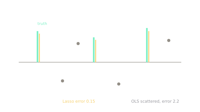
Take $d = 1000$ , $s = 10$ , $\sigma = 1$ and $n = 1500$ . Then $\log d = \ln 1000 \approx 6.91$ , $s\log d/n = 10 \times 6.91/1500 \approx 0.0461$ , and its square root is $\sqrt{0.0461} \approx 0.215$ . With constants near $0.7$ the bound lands near $0.15$ . So $1{,}500$ samples pin $10$ active coefficients among $1{,}000$ within $0.15$ Euclidean error.

Least squares cannot even start at $n = 200 < d$ : its variance term scales like $\sigma\sqrt{d/n} = \sqrt{5} \approx 2.24$ even where defined via pseudoinverse, an order above the Lasso error and with no selection. The $\log d$ price of $6.91$ replaces the $d$ price of $1{,}000$ , a $145$ -fold saving in effective dimension.

Watch Out For

Running Lasso with unnormalised columns

If one feature spans $0$ to $1000$ and another spans $0$ to $1$ , the same $\lambda$ punishes their coefficients unequally: the wide feature looks cheap per unit effect. Selection then favours scale, not signal, and the rate collapses.

Fix: standardise every column to unit $L_2$ or unit variance before fitting. Undo the scaling only when reporting.

Reading selected variables as the true support

Lasso selection is consistent only under an irrepresentability condition limiting correlations between active and inactive features. With strong correlations it swaps members, keeps proxies and drops truth while predicting well. Treating the selected set as discovered biology or causal drivers overclaims.

Fix: separate prediction from selection. For support claims use stability selection or debiased intervals, not the raw Lasso active set.

The Quick Version

With $d \ge n$ , structure is mandatory and sparsity plus $L_1$ is the standard structure.
Lasso error scales as $\sqrt{s\log d/n}$ , so 10 in 1000 need about 1500 samples for error 0.15.
Penalty near $\sigma\sqrt{\log d/n}$ with normalised columns; the design needs a restricted eigenvalue.
Least squares scales as $\sqrt{d/n}$ and is undefined below $d$ samples.
Selection needs stronger correlation conditions than prediction, so do not read support as truth.