Importance and Rejection Sampling

Hard distributions are sampled through easy ones. Rejection throws away the mismatches, while importance keeps everything and reweights it.

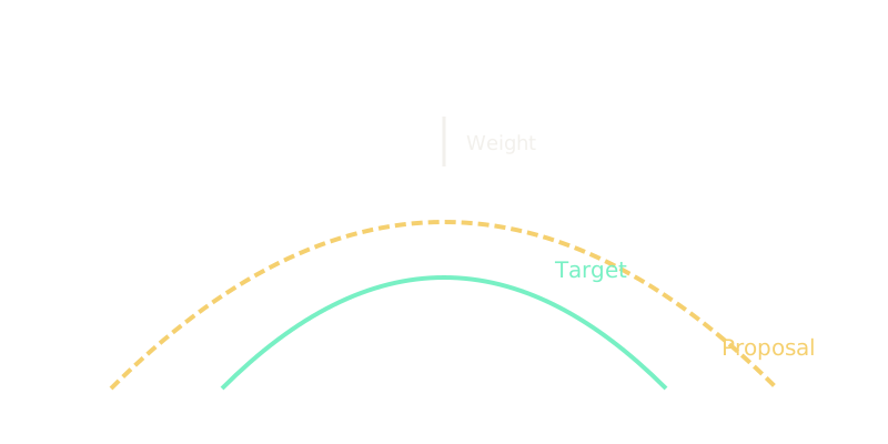
A uniform proposal with envelope M 1.5 covers target 0.2, 0.5, 0.3 and weights 0.6, 1.5, 0.9 recover mean 2.1.

Why Does This Exist?

Many distributions cannot be sampled directly. A posterior over parameters or a rare-event model has a density we can evaluate but no direct sampler, yet Monte Carlo averages need draws from exactly it. Drawing from the wrong distribution and averaging naively answers the wrong question.

Two corrections fix the mismatch. Rejection sampling draws from an easy proposal inside an envelope and discards draws that fall above the target. Importance sampling keeps every draw and multiplies it by $p/q$ . Both rest on integrals in probability, resampling ideas in bootstrap, and they motivate gradient-friendly samplers like Hamiltonian Monte Carlo.

The one idea you need first

Expectations are integrals. The mean of $f$ under $p$ is $\sum f(x) p(x)$ in discrete form. If draws come from $q$ instead, multiplying each term by $p(x)/q(x)$ restores the $p$ integral, provided $q(x) > 0$ wherever $p(x) > 0$ .

Think of It Like This

Counting fish with a biased net

A net catches big fish twice as often as their share in the lake. Throwing back catches by a rule restores fairness: keep a small fish always, keep a big one only half the time. That is rejection. Alternatively keep everything but count each big fish as half a fish in the tally. That is importance weighting.

It stops at support. If the net mesh lets every minnow escape, no rerule or reweight recovers them. The proposal must reach everywhere the target lives.

How It Actually Works

Pick a proposal $q$ that is easy to sample with $q(x) > 0$ wherever $p(x) > 0$ . For rejection, find $M$ with $p(x) \le M q(x)$ for all $x$ . Draw $x$ from $q$ and $u$ uniform in $[0, 1]$ , and accept when $u \le p(x) / (M q(x))$ . Accepted draws follow $p$ exactly, and the overall acceptance rate is $1/M$ .

For importance, skip $M$ . Draw $x_1, \dots, x_n$ from $q$ and weight each by $w(x) = p(x)/q(x)$ . Then $\sum f(x_i) w(x_i) / \sum w(x_i)$ estimates the mean of $f$ under $p$ . In plain words: $q$ proposes, $w$ corrects, $M$ prices rejection.

Worked example

Values $\{1, 2, 3\}$ have target $p = [0.2, 0.5, 0.3]$ and uniform proposal $q = [1/3, 1/3, 1/3]$ with $1/3 \approx 0.333$ .

Weights are $w = p/q$ . For $1$ : $0.2 / 0.333 = 0.6$ . For $2$ : $0.5 / 0.333 = 1.5$ . For $3$ : $0.3 / 0.333 = 0.9$ . So $w = [0.6, 1.5, 0.9]$ .

The envelope constant is the largest weight: $M = 1.5$ . Then $M q = [0.5, 0.5, 0.5]$ , which covers $p = [0.2, 0.5, 0.3]$ entry by entry. Per-value acceptance is $p/(Mq)$ : $[0.2/0.5, 0.5/0.5, 0.3/0.5] = [0.4, 1.0, 0.6]$ . Overall acceptance is $1/M = 1/1.5 \approx 0.667$ , so about two of three proposals survive.

The true mean is $1 \times 0.2 + 2 \times 0.5 + 3 \times 0.3 = 0.2 + 1.0 + 0.9 = 2.1$ . The importance form with exact weights gives $1 \times 0.6 + 2 \times 1.5 + 3 \times 0.9 = 0.6 + 3.0 + 2.7 = 6.3$ , divided by $0.6 + 1.5 + 0.9 = 3.0$ , which is $6.3/3.0 = 2.1$ . The diagram draws these three weights beside the $M = 1.5$ envelope.

Code

The point is the correction factor. Unweighted proposal draws average to $2.0$ , while the $p/q$ weights move the answer to $2.1$ .

1import numpy as np2
3
4def importance_weights(p: np.ndarray, q: np.ndarray) -> np.ndarray:5    return p / q  # q must be positive wherever p is positive6
7
8p = np.array([0.2, 0.5, 0.3])9q = np.array([1.0 / 3, 1.0 / 3, 1.0 / 3])10w = importance_weights(p, q)11print(np.round(w, 2))  # -> [0.6 1.5 0.9]12vals = np.array([1.0, 2.0, 3.0])13print(float(np.sum(vals * w) / np.sum(w)))  # -> 2.114print(float(1.0 / np.max(w)))  # -> 0.6666666666666666

The last line is $1/M$ : two of three proposals accepted on average, matching the hand rate of $0.667$ .

Watch Out For

Proposing zero where the target is positive

If $q(x) = 0$ while $p(x) > 0$ , the weight $p/q$ divides by zero and rejection can never propose that $x$ . The symptom is a confidently wrong mean: the missing region never appears, variance estimates look small, and more draws do not fix it. Check support first, and fatten proposal tails until every target region gets samples.

Setting M below the true maximum

Rejection needs $M q$ above $p$ everywhere, but the maximum ratio is often guessed from a short pilot run. Too-small $M = 1.2$ when the truth needs $1.5$ over-accepts the peak at $x = 2$ and biases the sample toward it. The symptom is a sampler that looks efficient because it rarely rejects, yet histograms pile up at the mode. Track the largest observed $p/q$ and add margin, or switch to importance weights which need no $M$ .

The Quick Version

Proposal $q$ draws, weight $w = p/q$ corrects, envelope $M$ enables rejection.
Here $p = 0.2, 0.5, 0.3$ with uniform $q$ gives weights $0.6, 1.5, 0.9$ .
Envelope needs $M = 1.5$ , acceptance is $1/M \approx 0.667$ , per-value rates are $0.4, 1.0, 0.6$ .
Weighted mean is $6.3/3.0 = 2.1$ , exactly the target mean.
Missing support cannot be reweighted back, and too-small $M$ biases toward the mode.