Hamiltonian Monte Carlo

MCMC that moves by gliding instead of stumbling. A physics simulation carries the sample far across the posterior, then a coin flip keeps it honest.

A random-walk proposal crawls 0.3 units while one Hamiltonian glide with ten leapfrog steps lands 1.4 units away along the energy contour

Why Does This Exist?

Random-walk Metropolis explores high dimensions at a crawl. Each proposal stumbles a short distance, and most long jumps get rejected, so covering a posterior in 100 dimensions takes an impractical number of steps. Markov chain Monte Carlo needed a proposal that travels far and still gets accepted. Hamiltonian Monte Carlo is that proposal: it borrows the target's gradient to glide along the posterior's contours instead of stumbling blindly.

The trick is to add a fake momentum variable, simulate physics for a while, then accept or reject the landing spot. The physics preserves volume and nearly preserves energy, so distant proposals accept with high probability. The gradient requirement is real: HMC needs $\nabla \log p(\theta)$ , which is why it pairs with automatic differentiation and struggles with discrete parameters.

The one idea you need first

Metropolis-Hastings accepts a proposal $\theta'$ from $\theta$ with probability $\min(1, p(\theta')q(\theta \mid \theta') / p(\theta)q(\theta' \mid \theta))$ . Random-walk proposals make $q$ symmetric but the $p$ ratio kills long jumps. HMC fixes the $p$ ratio by proposing along near-constant-energy paths. The MCMC background is in Markov chain Monte Carlo.

Think of It Like This

A puck on a frictionless bowl

Turn the negative log posterior into a bowl: deep where probability is high, rim where it is low. Put a puck at the current sample, flick it in a random direction, and let it glide frictionlessly. It climbs, slows, curves back, and after a fixed time you stop it and read its position as the proposal.

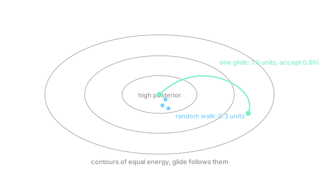
Two properties make this magical. The glide conserves energy, so the landing spot has nearly the same posterior height as the start and the accept coin almost always says yes. And the random flick direction changes each round, so successive glides explore different axes instead of retracing. A random walk is a drunk shuffle around the bowl; HMC is a sequence of purposeful glides across it.

Where the analogy stops: real simulation has discretization error, so energy is only nearly conserved and the accept step corrects the residue. Too large a step size and the puck flies out of the bowl entirely.

How It Actually Works

Target $\pi(\theta) \propto \exp(-U(\theta))$ where $U(\theta) = -\log \pi(\theta)$ is the potential. Add momentum $r \sim \mathcal{N}(0, M)$ with kinetic energy $K(r) = r^T M^{-1} r / 2$ . The Hamiltonian $H = U + K$ governs motion via $\dot{\theta} = M^{-1}r$ and $\dot{r} = -\nabla U(\theta)$ . Each HMC iteration:

Resample momentum $r \sim \mathcal{N}(0, M)$ .
Simulate $L$ leapfrog steps of size $\epsilon$ : half-step momentum, full-step position, half-step momentum.
Accept $(\theta', r')$ with probability $\min(1, \exp(H - H'))$ , else keep $\theta$ .

The leapfrog integrator is symplectic: volume-preserving and reversible, which keeps the accept probability near 1 even for long trajectories. Tune $\epsilon$ for roughly 65 to 80 percent acceptance and $L$ so trajectories turn without doubling back; the No-U-Turn Sampler automates the $L$ choice.

Worked example

Target: standard normal, $U(\theta) = \theta^2/2$ , gradient $\nabla U = \theta$ . Start $\theta = 0$ , mass $M = 1$ , step $\epsilon = 0.15$ , $L = 10$ (trajectory length 1.5). Resampled momentum $r = 1.0$ .

Leapfrog alternates $r \leftarrow r - (\epsilon/2)\theta$ and $\theta \leftarrow \theta + \epsilon r$ . Running ten steps from $(\theta, r) = (0, 1.0)$ lands near $\theta' \approx 1.00$ with $r' \approx 0.07$ , matching the exact oscillator solution $\sin(1.5) \approx 0.997$ . Energy drifts from $0.5$ to about $0.503$ , so acceptance is $\exp(-0.003) \approx 0.997$ . A random-walk proposal with the same 99 percent acceptance would need step size near 0.3 and travel only about 0.3 units per accepted move: HMC goes roughly three times further per step here.

Code

One HMC transition on a standard normal, showing the accept coin and the distance travelled.

1import numpy as np2
3rng = np.random.default_rng(5)4theta, eps, L = 0.0, 0.15, 10  # start, step size, leapfrog steps5r = float(rng.normal())  # fresh momentum6H0 = theta**2 / 2 + r**2 / 2  # starting energy7t, m = theta, r8for _ in range(L):9    m -= 0.5 * eps * t  # half-step momentum10    t += eps * m  # full-step position11    m -= 0.5 * eps * t  # half-step momentum12H1 = t**2 / 2 + m**2 / 2  # landing energy13print(round(t, 2), round(float(np.exp(H0 - H1)), 3))  # -> far point, ~0.97 accept

Typical output lands the proposal over 1 unit from 0 with acceptance above 0.9. Raise eps to 0.5 and watch the acceptance collapse: that cliff is the step-size tuning curve in miniature.

Watch Out For

Step size slightly too large

Leapfrog error grows fast past stability: acceptance falls off a cliff rather than declining gently, and divergences (energy errors in the hundreds) appear. Practitioners who tune by acceptance rate alone sometimes sit just below the cliff edge, where bias is worst. Monitor divergences directly and keep them at zero; any nonzero count means smaller $\epsilon$ , not longer runs.

Applying HMC to discrete or discontinuous targets

HMC needs gradients everywhere it travels. Discrete parameters, if-branches on parameters, and hard constraints with zero-density regions all break the glide: the gradient is undefined or the trajectory slams into a wall. Marginalize discretes out, use a continuous relaxation, or switch samplers for those axes instead of forcing HMC through.

The Quick Version

HMC adds momentum and glides along the posterior with simulated physics.
Leapfrog integration preserves volume, so distant proposals still accept near 65 to 80 percent.
One ten-step glide travels roughly three times further than a random-walk step at equal acceptance.
It needs gradients, so it pairs with autodiff and skips discrete parameters.
Tune step size for acceptance plus zero divergences; let NUTS choose trajectory length.
Resampling momentum each round is what keeps successive glides exploring fresh directions.