Learning Rate Schedules

Why Does This Exist?

One fixed step size cannot serve a whole training run. Early steps start from random weights where large updates can blow up activations, while late steps near a minimum need small updates because the same large step bounces across the valley instead of settling. A single rate either crawls early or rattles late.

Schedules resolve the tension by varying the learning rate $\eta$, where $\eta$ multiplies the gradient in the update $w \leftarrow w - \eta \nabla f$. Warmup ramps gently to protect early steps, step decay drops in stages to spend most time at productive mid-range rates, and cosine annealing glides smoothly to zero for a clean finish. The batch-size choice around those steps lives in gradient descent variants, per-coordinate adaptation lives in stochastic gradient descent variants, and the convex landscape where decay guarantees most lives in convex optimization.

The prerequisite is the gradient update itself: the gradient points uphill, so training subtracts a scaled copy. When that picture is fuzzy, read gradients first.

Think of It Like This

How It Actually Works

Write $\eta_t$ for the learning rate at epoch $t$, where $t$ counts completed passes over the data. All three schedules below share endpoints $0.1$ and $0$ over different shapes, so the diagram compares shape rather than scale.

Warmup then decay

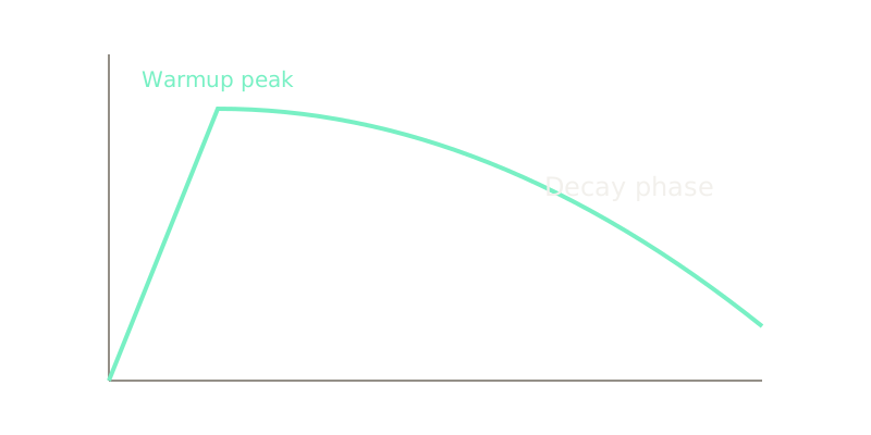
Linear warmup over $W = 5$ epochs from 0 to $\eta_{\max} = 0.1$ is $\eta_t = 0.1 \times t / 5$ for $t < 5$. The hand values are epoch 0 at 0, epoch 1 at 0.02, epoch 2 at 0.04, epoch 3 at 0.06, epoch 4 at 0.08, and epoch 5 at 0.1. Early variance is highest when weights are random and optimizer statistics are empty, so starting near zero avoids one giant destructive first step, especially with large batches and transformers.

Step decay

Step decay holds a rate constant, then multiplies by $\gamma = 0.5$ at milestones 30, 60, and 90. From 0.1 the hand values are 0.1 before epoch 30, 0.05 from epoch 30, 0.025 from epoch 60, and 0.0125 from epoch 90. Each drop cuts bounce roughly in half while keeping the implementation to two numbers. The cost is the cliff itself: a drop before the run has exploited the current scale wastes the remaining budget at too-small steps.

Cosine annealing

Cosine annealing over $T = 100$ epochs from $\eta_{\max} = 0.1$ to 0 is $\eta_t = 0.05 \times (1 + \cos(\pi t / 100))$, where $\cos$ is the cosine function and $\pi$ the half-period constant. The hand values are epoch 0 at 0.1, epoch 50 at 0.05, and epoch 100 at 0. The curve falls slowly at both ends and fastest in the middle, spending little time at the destructive top and arriving flat at the bottom. After warmup the same curve restarts from the warmed peak, which is why pipelines pair the two.

Worked example

Fix $T = 100$ and $\eta_{\max} = 0.1$ for all three. Warmup reaches 0.1 exactly at epoch 5. Step decay reads 0.1, 0.05, 0.025, and 0.0125 across milestones 0, 30, 60, and 90. Cosine reads 0.1 at epoch 0, 0.05 at epoch 50, and 0 at epoch 100, since $\cos(0) = 1$, $\cos(\pi/2) = 0$, and $\cos(\pi) = -1$. The diagram draws exactly these four curves from the shared start $(0, 0.1)$ to the shared end $(100, 0)$, so shape is the only difference on display.

Code

The snippet evaluates the three shapes with only the standard library.

1import math2
3
4def cosine(t: int, total: int = 100) -> float:5    return 0.05 * (1 + math.cos(math.pi * t / total))6
7
8def step_decay(t: int) -> float:9    lr = 0.110    if t >= 30:11        lr *= 0.512    if t >= 60:13        lr *= 0.514    if t >= 90:15        lr *= 0.516    return lr17
18
19print(round(cosine(0), 4))  # -> 0.120print(round(cosine(50), 4))  # -> 0.0521print(round(cosine(100), 4))  # -> 0.022print(step_decay(0), step_decay(30), step_decay(60), step_decay(90))  # -> 0.1 0.05 0.025 0.012523print(round(0.1 * 3 / 5, 4))  # -> 0.06

Cosine passes through 0.1, 0.05, and 0.0, step decay halves on schedule, and warmup hits 0.06 at epoch 3, matching the hand values above.

Watch Out For

The Quick Version

• One fixed rate cannot cover random starts and sharp finishes, so the rate becomes a schedule over epochs.
• Linear warmup ramps 0 to 0.1 across the first 5 epochs to protect early steps.
• Step decay halves 0.1 to 0.05 to 0.025 to 0.0125 at epochs 30, 60, and 90.
• Cosine annealing glides 0.1 through 0.05 at epoch 50 to 0 at epoch 100 with no cliffs.
• Pair warmup with a decay shape rather than running either alone.
• Time decays against validation plateaus, because early decay strands the run.

What to Read Next

• Gradient Descent Variants
• SGD and Optimization Variants
• Convex Optimization