Lebesgue Measure

A consistent rule for length, area and volume that handles the jagged sets Riemann sums cannot, by covering instead of partitioning.

Why Does This Exist?

Riemann integration chops the domain into intervals and works while functions are tame. It breaks on sets like the rationals in $[0,1]$ : every interval contains both rational and irrational points, so upper and lower sums never meet. Probability needs better, because events are sets and "probability zero" must be meaningful for uncountable outcomes.

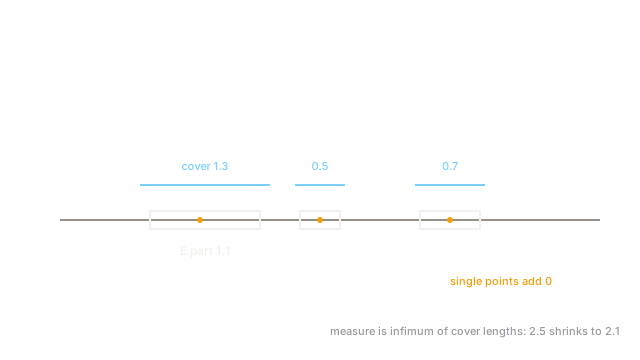
Lebesgue measure fixes the ruler first. Cover a set by intervals, add their lengths, and take the infimum over all covers. Countable points contribute nothing, which is why single outcomes can have probability zero without being impossible.

This page builds the ruler. Using it to integrate is in Lebesgue integration, and the probability reading is in measure spaces.

The one idea you need first

Length of an interval $[a,b]$ is $b - a$ . Outer measure extends this by covering any set $E$ with intervals $I_k$ and taking $\inf \sum \ell(I_k)$ . Measurable sets are those where the cover splits cleanly.

Think of It Like This

Wrapping odd shapes in cling film

You want the area of spilled paint with holes and specks. Instead of cutting it into grid squares, you wrap each blob in rectangular film and add the film areas, trimming until the wrap hugs the paint.

The film is the interval cover. Trimming is the infimum. Dust specks need almost no film, which is why countable sets get measure zero. Where the analogy stops: film always overestimates; measure theory proves the infimum is consistent across different wrappings.

How It Actually Works

Outer measure $m^*(E) = \inf \{\sum \ell(I_k) : E \subset \cup I_k\}$ . A set $E$ is Lebesgue measurable when for every test set $A$ , $m^*(A) = m^*(A \cap E) + m^*(A \setminus E)$ . Lebesgue measure $m$ is $m^*$ restricted to measurable sets. It is countably additive: $m(\sqcup E_k) = \sum m(E_k)$ for disjoint measurable $E_k$ .

A null set has $m(E) = 0$ . Countable sets are null: cover the $k$ -th point by an interval of length $\epsilon/2^k$ ; total $\le \epsilon$ for any $\epsilon > 0$ . Properties holding outside a null set hold almost everywhere.

Worked example

Measure of $[0,1]$ is $1$ . The rationals $\mathbb{Q} \cap [0,1]$ are countable: enumerate $q_1, q_2, \ldots$ and cover $q_k$ with length $0.01/2^k$ . Total cover $0.01$ , so $m^* \le 0.01$ . Since $\epsilon$ was arbitrary, measure $0$ . The irrationals then have measure $1 - 0 = 1$ . Riemann cannot separate the two; Lebesgue does.

Watch Out For

Treating all sets as measurable

Symptom: assuming countable additivity for arbitrary unions and deriving contradictions like $1 = 0$ on quotient sets. Fix: check measurability first; non-measurable Vitali sets need choice and never appear in ML practice.

Reading measure zero as impossible

Symptom: discarding a density value at one point because "probability zero means it cannot happen". Fix: points have zero measure but positive density; only null events with structure, not single continuous outcomes, carry the impossibility reading.

The Quick Version

Lebesgue measure extends interval length by cheapest covering, then restricts to sets that split cleanly.
It is countably additive on measurable sets, which Riemann sums are not.
Countable sets have measure zero; rationals in $[0,1]$ measure $0$ while irrationals measure $1$ .
Null sets make "almost everywhere" and "almost surely" precise.
Non-measurable sets exist but never occur in practical modelling.