Math

Bayesian Inference

Keep the whole distribution over parameters instead of one best guess, so the model can report how much it does not know — and pay for it with an integral that has to be dodged rather than solved.

Why Does This Exist?

Because a softmax output of 0.97 tells you nothing about whether the model has any business being confident.

A trained network gives you one set of weights and, from them, one probability per class. That number reflects aleatoric uncertainty — genuine ambiguity in the data, a blurred image, a coin flip. It says nothing about epistemic uncertainty: whether the training data ever contained anything like this input. The two are different questions and a point estimate collapses them into one number. This is why a classifier shown a photograph of static returns 0.97 for "golden retriever" and why that is not a bug you can fix inside the softmax.

Bayesian inference keeps the whole distribution over parameters, so it can distinguish "the answer is genuinely uncertain" from "I have never seen anything like this". Four things depend on that distinction:

Active learning selects the examples the model is uncertain about because it lacks data, which is epistemic uncertainty specifically. Selecting on softmax confidence instead picks the genuinely ambiguous examples, which are the ones labelling will not help.
Out-of-distribution detection in anything safety-relevant — medical triage, autonomous control, fraud escalation — is an epistemic-uncertainty question.
Thompson sampling, the strongest simple answer to the explore–exploit problem in bandits and recommenders, works by drawing a parameter from the posterior and acting as though it were true. There is nothing to draw from without a posterior.
Small-data decisions. With forty examples, a point estimate plus a p-value is a weaker and more brittle summary than a posterior you can integrate over.

There is also a debt this page settles. MAP estimation already gave you the posterior's peak. This page is what the rest of the posterior was for.

Think of It Like This

Two weather forecasters, one of whom admits what they do not know

Forecaster A says: "70% chance of rain." Every day. One number, always.

Forecaster B says: "70% chance of rain, and I am confident — this is a familiar pattern, I have seen a thousand days like it." Or on a different day: "70% chance of rain, but honestly this system is unlike anything in my records; treat that number as roughly a coin flip with extra steps."

Both give you 70%. Only one gives you enough to act on. If you are deciding whether to cancel an outdoor event, A's 70% and B's two different 70%s should lead to different decisions, and A has withheld the information you need.

Forecaster B is doing Bayesian inference. The extra thing being carried is a distribution over what the right answer might be, not just its centre.

Three properties of the analogy hold precisely:

Confidence comes from data volume, not from the prediction's value. B's uncertainty is about how much relevant evidence exists, which is independent of whether the answer is 70% or 20%. This is exactly the aleatoric–epistemic split.

Prior knowledge is legitimate input. B knows things about weather that are not in this week's observations. A Bayesian model states that knowledge explicitly, as a prior, where it can be argued with — rather than smuggling it in through architecture choices and hyperparameters, where it cannot.

Being calibrated is not the same as being right. B can be well calibrated and still wrong on any given day. Uncertainty quantification tells you how much to trust a prediction; it does not improve the prediction.

Where the analogy stops: a real forecaster narrows their uncertainty by thinking. A Bayesian model narrows it by an integral over every possible parameter setting, and for anything with more than a handful of parameters that integral cannot be computed. Everything difficult about this page is downstream of that.

How It Actually Works

The mechanism is Bayes' theorem with parameters $\theta$ in the unknown slot:

p(\theta \mid D) = \frac{p(D \mid \theta)\, p(\theta)}{p(D)}

Four named pieces, and the discipline of naming them is most of the skill:

Prior $p(\theta)$ — what you believed before the data.
Likelihood $p(D \mid \theta)$ — how well each candidate parameter explains the data. This is the same function maximum likelihood maximises.
Posterior $p(\theta \mid D)$ — the belief afterwards. This, not a number, is the output.
Evidence $p(D) = \int p(D \mid \theta)\, p(\theta)\, d\theta$ — the normaliser, and the reason this page is hard.

The evidence is an integral over the entire parameter space. For a model with millions of parameters it is not slow, it is impossible, and every practical method below is a way of not computing it.

What you do with a posterior

Three things, and the third is the one that matters for prediction.

Summarise it. Its mean is the standard point estimate — and note it is not the mode, so it is not the MAP estimate. Its standard deviation is your uncertainty. A credible interval is the range containing 95% of the posterior mass, and it means what people wrongly believe a confidence interval means: there is a 95% probability the parameter is in there, given this model and prior. That difference is the single clearest practical distinction between the two traditions.

Sample from it. Draw a plausible parameter setting and act on it. This is Thompson sampling in one sentence.

Integrate over it to predict. Rather than predicting with one $\theta$ , average the predictions of every $\theta$ , weighted by how plausible it is:

p(y^* \mid x^*, D) = \int p(y^* \mid x^*, \theta)\, p(\theta \mid D)\, d\theta

In plain words: ask every plausible model what it thinks and average the answers, weighting each by its posterior probability. This is the predictive distribution, and it is where calibration comes from — when the plausible models disagree, the averaged prediction is appropriately unsure, automatically.

That integral is also the honest description of what a deep ensemble is doing. Five independently trained networks are five samples from something posterior-like, and averaging their predictions is a crude Monte Carlo estimate of the integral above. Ensembles are the most reliable uncertainty method in deep learning, and this is why they work.

The four ways around the evidence integral

Conjugate priors — solve it exactly. For certain prior–likelihood pairs the posterior is in the same family as the prior and the update is arithmetic on counts. Beta prior with binomial likelihood gives a Beta posterior. Gaussian with known variance gives a Gaussian. Dirichlet with multinomial gives a Dirichlet. Exact, instant, and available only for these handful of pairs — but they cover A/B tests, click-through rates and bandit arms, which is a large fraction of the Bayesian work actually done in industry.

MAP — take the peak and skip the integral. The denominator does not depend on $\theta$ , so the mode needs no normaliser. Cheap, and what regularised training already does. You lose the uncertainty entirely.

Monte Carlo — sample without normalising. MCMC constructs a chain whose stationary distribution is the posterior, and remarkably it needs only ratios of posterior densities, in which the unknown normaliser cancels. Asymptotically exact, and too slow for a large network. Covered in Monte Carlo methods.

Variational inference — optimise a bound. Replace the true posterior with a tractable family $q_\phi(\theta)$ , usually independent Gaussians, and fit $\phi$ by maximising the ELBO:

\mathcal{L}(\phi) = \mathbb{E}_{q_\phi}\big[\log p(D \mid \theta)\big] - D_{\mathrm{KL}}\big(q_\phi(\theta) \,\big\|\, p(\theta)\big)

In plain words: fit the data, minus a penalty for drifting from the prior. It is a lower bound on the log evidence, guaranteed by the non-negativity of KL divergence, and the gap is exactly the KL divergence from $q$ to the true posterior. This is a gradient-descent problem, which is why it scales — and it is verbatim the VAE objective, with $\theta$ being per-datapoint latents rather than weights.

The trade is the usual one: conjugate is exact and narrow, MCMC is exact and slow, variational is fast and biased. The bias has a direction, and it is knowable: variational inference minimises the reverse KL, which is mode-seeking, so a variational posterior is characteristically too narrow. It will under-report uncertainty, which is the wrong direction for a method whose entire purpose is reporting uncertainty.

Worked example

A coin, because the Beta–Binomial pair is conjugate and every step is checkable.

Start with a $\mathrm{Beta}(2, 2)$ prior — mild belief in fairness, worth one pseudo-head and one pseudo-tail. Flip ten times, get three heads and seven tails. The conjugate update is addition:

\text{posterior} = \mathrm{Beta}(2 + 3,\ 2 + 7) = \mathrm{Beta}(5, 9)

That is the entire inference. No integral, no sampling. Now read the answers off the posterior, using $\mathrm{Beta}(\alpha,\beta)$ having mean $\alpha/(\alpha+\beta)$ and mode $(\alpha-1)/(\alpha+\beta-2)$ :

\text{mean} = \frac{5}{14} = 0.357, \qquad \text{mode} = \frac{4}{12} = 0.333, \qquad \text{sd} = 0.124

Three separate points worth making from three numbers:

The mode 0.333 is the MAP estimate from the previous page. It is one summary of this posterior, and not the one you would usually report.
The mean 0.357 differs from the mode, because the posterior is skewed. With ten observations that skew is real, and quoting the mode as "the estimate" understates the bias.
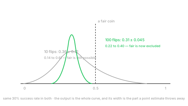
The standard deviation 0.124 is the answer a point estimate cannot give. Roughly, the bias is $0.36 \pm 0.12$ . A 95% credible interval runs from about 0.14 to 0.61 — this coin might be badly biased or might be fair, and ten flips genuinely cannot tell.

Now the same 30% rate with ten times the data: 100 flips, 30 heads.

\text{posterior} = \mathrm{Beta}(32, 72), \qquad \text{mean} = \frac{32}{104} = 0.308, \qquad \text{sd} = 0.045

The mean has slid from 0.357 to 0.308, almost onto the observed 0.30, because four pseudo-observations against a hundred real ones barely register. And the standard deviation has fallen from 0.124 to 0.045 — a factor of 2.75 for ten times the data, which is the $1/\sqrt{n}$ law showing up ( $\sqrt{10} = 3.16$ , and the small shortfall is the prior still contributing). The credible interval is now roughly 0.22 to 0.40, which excludes 0.5. Ten flips could not rule out a fair coin; a hundred can.

Notice what the posterior did that no point estimate could: it changed shape. Both datasets have a 30% success rate, and the conclusion you can draw from them is completely different.

Show Me the Code

1import numpy as np2from scipy import stats3
4
5def beta_posterior(heads: int, n: int, a0: float, b0: float) -> stats.rv_continuous:6    """Conjugate update: the Beta prior's parameters just absorb the counts."""7    return stats.beta(a0 + heads, b0 + n - heads)8
9
10for heads, n in ((3, 10), (30, 100)):11    post = beta_posterior(heads, n, 2, 2)                     # Beta(2,2) prior12    lo, hi = post.interval(0.95)                              # 95% credible interval13    print(n, round(post.mean(), 3), round(post.std(), 3), np.round([lo, hi], 2))14# -> 10  0.357 0.124 [0.14 0.61]      wide: cannot rule out a fair coin15# -> 100 0.308 0.045 [0.22 0.4 ]      narrow, and 0.5 is now excluded16
17post = beta_posterior(3, 10, 2, 2)18print(round(float(post.cdf(0.5)), 3))          # -> 0.867  P(coin favours tails)19print(round(float(np.mean(post.rvs(100_000, random_state=0) > 0.4)), 3))  # -> 0.354

The last two lines are the payoff a point estimate cannot reach. cdf(0.5) answers "what is the probability this coin favours tails" directly — 0.867, likely but far from settled — and the sampled line answers an arbitrary question, "is the bias above 0.4", by drawing 100,000 parameters from the posterior and counting. Any question you can phrase about $\theta$ becomes an integral you can estimate this way.

Watch Out For

Reporting a posterior without saying what prior produced it

A posterior is a function of the data and the prior, and with limited data the prior can be doing most of the work. A credible interval quoted without its prior is not reproducible and not checkable.

The failure has a shape. Someone picks a prior that looks harmless, gets a narrow posterior, and reports a confident conclusion that is mostly the prior talking. Two ways this happens with priors nobody flagged as strong:

A "non-informative" prior that is not. A $\mathrm{Uniform}(0,1)$ prior on a probability is flat and feels neutral. Reparameterise to log-odds and it is not flat at all — it concentrates mass away from the extremes. Flatness is not a property of a belief, it is a property of a belief in a particular parameterisation, and it does not survive a change of variables. Jeffreys priors exist precisely to be invariant under reparameterisation, and for a proportion the Jeffreys prior is $\mathrm{Beta}(0.5, 0.5)$ rather than $\mathrm{Beta}(1,1)$ .

A wide prior that is secretly strong. A $\mathcal{N}(0, 100^2)$ prior on a logistic-regression coefficient sounds vague. On the log-odds scale it asserts that odds ratios of $e^{200}$ are plausible, which puts almost all its mass on effects so extreme they predict every outcome with certainty. In practice this prior drags estimates outward and makes separation problems worse. The recommended default for logistic coefficients on standardised features is around $\mathcal{N}(0, 2.5^2)$ , which is far tighter than "vague" suggests.

What to do:

Report the prior alongside the posterior. Always, in one line.
Run a prior sensitivity check. Redo the inference with two or three defensible priors. If the conclusion holds, say so; if it flips, the data is not carrying the argument and no amount of presentation fixes that.
Do a prior predictive check. Sample parameters from the prior, generate fake data, and look at it. If your prior generates patients 400 years old or click-through rates of 0.9999, it is not vague, it is wrong.
Prefer weakly informative priors that rule out the absurd while staying agnostic about the plausible.

Trusting a variational posterior's width, or an unconverged chain's samples

Both approximate methods fail quietly, returning plausible-looking numbers with no error raised.

Variational inference under-reports uncertainty, systematically. It minimises the reverse KL divergence, which is mode-seeking, so it finds one mode of the posterior and reports that mode's width as the whole uncertainty. Add the usual mean-field assumption — independent Gaussians, no correlations between parameters — and correlated parameters have their joint uncertainty discarded as well. The result is a posterior that is too narrow, sometimes by a large factor, on a method you deployed in order to know what you do not know. The practical implication for Bayesian neural networks is direct: a mean-field variational network's uncertainty estimate is usually worse than a five-member deep ensemble's, at comparable cost. Reach for the ensemble first.

MCMC returns samples whether or not it has converged. A chain stuck in one region produces a tight, confident, wrong posterior, and nothing in the output says so. The diagnostics are not optional:

$\hat{R}$ (R-hat) compares variance between chains to variance within them. Run at least four chains from different starts and require $\hat{R} < 1.01$ . A single chain cannot produce this statistic, which is the reason to run several.
Effective sample size. Consecutive MCMC draws are correlated, so 10,000 samples may carry the information of 200. Below about 400 effective samples per parameter, the tail quantiles of your credible interval are noise.
Divergences, in Hamiltonian samplers like NUTS. Any non-zero count means the geometry defeated the sampler and the affected region is under-explored. Reparameterise — the non-centred parameterisation for hierarchical models is the standard fix — rather than raising the step-size target and hoping.

The unifying point: for both methods, the failure mode is a posterior that is too narrow. A method whose errors always point toward overconfidence needs its diagnostics run every time, not once during development.

The Quick Version

Bayesian inference produces a posterior distribution over parameters, not a point estimate.
Prior times likelihood, divided by the evidence. The evidence is an integral over all parameters and is the source of every difficulty.
The posterior separates aleatoric uncertainty (the data is ambiguous) from epistemic uncertainty (there was no relevant data), which a softmax cannot do.
Predict by integrating over the posterior, not by picking one $\theta$ . A deep ensemble is a crude version of exactly this integral.
A credible interval means what people wrongly think a confidence interval means: 95% posterior probability the parameter is inside.
Four routes around the evidence: conjugate priors (exact, narrow), MAP (cheap, no uncertainty), MCMC (exact, slow), variational (fast, biased narrow).
The ELBO is a lower bound on the log evidence, guaranteed by KL non-negativity, and is verbatim the VAE objective.
Always report the prior. "Non-informative" is not a property that survives reparameterisation, and a wide prior on log-odds can be very strong.
Variational posteriors are too narrow by construction; unconverged MCMC is too narrow silently. Check $\hat{R}$ , effective sample size and divergences.