Multivariate Distributions

One variable's distribution is a profile. Several variables together form a landscape, and the covariance matrix maps how its hills lean on each other.

A mosaic of the joint table with column widths from X and inner splits from Y given X shows the dependence as uneven rows and a covariance of 0.1

Why Does This Exist?

Single-variable distributions describe one measurement at a time, but data arrives in rows: features together, pixels together, a whole embedding at once. Treating each column separately discards exactly what models need most, how the columns move together. Correlated features break naive assumptions, joint structure is what classifiers exploit, and sampling realistic synthetic data means reproducing the togetherness, not just the profiles.

A multivariate distribution is the joint law of a whole vector: one rule weighing every combination. Its two organizers are the mean vector, collecting the centers, and the covariance matrix, mapping every pairwise lean. The single-variable machinery is probability distributions and the averaging behind it is expectation, variance and covariance; this page assembles them into the vector picture.

The one idea you need first

A random vector stacks several random variables into one object $X = (X_1, \ldots, X_d)$ . Its joint distribution answers combination questions: the chance that $X_1$ lands here and $X_2$ lands there. Projecting onto one coordinate by ignoring the rest gives a marginal distribution, and the dedicated slicing mechanics are taught in the joint, marginal and conditional distributions page.

Think of It Like This

A class photo versus individual portraits

Separate portraits show each student clearly but say nothing about friendships. The class photo shows who stands with whom: clusters, loners, the pair always side by side. Same students, extra information living purely in the arrangement.

Marginals are the portraits and the joint is the class photo. Two datasets can share every column profile yet tell opposite stories, one with study time tracking scores and one with them unrelated. The covariance matrix is the seating chart: which pairs lean together and how strongly. Models trained on portraits alone keep confusing the two classes, because the signal was in the arrangement all along.

The analogy stops at linearity. A seating chart records who stands near whom, and covariance likewise records only straight-line lean. Curved arrangements, circles and parabolas of dependence, need the fuller joint picture the mosaic below gestures at.

How It Actually Works

A bivariate distribution is fully shown by its joint table or density, and three summaries organize it:

The mean vector $\mu = (E[X], E[Y])$ : the center of mass in each direction. Expectation applies coordinate by coordinate.
The covariance matrix $\Sigma$ : variances on the diagonal, pairwise covariances off it. Entry $\Sigma_{ij} = E[(X_i - \mu_i)(X_j - \mu_j)]$ is positive when the pair rises together.
The correlation matrix: each covariance divided by both standard deviations, rescaling every lean into $[-1, 1]$ . Covariance speaks units; correlation speaks strength.

In plain words: the table holds everything, the mean vector centers it, the covariance matrix tilts it. Positive off-diagonals stretch the cloud along the rising diagonal, negative ones along the falling diagonal, and zeros mean the linear lean is gone, though curved dependence may remain.

Worked example

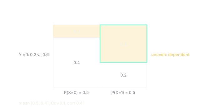
Toss two biased-together coins with joint chances $P(0,0) = 0.4$ , $P(0,1) = 0.1$ , $P(1,0) = 0.2$ , $P(1,1) = 0.3$ .

Marginals: $P(X = 1) = 0.2 + 0.3 = 0.5$ and $P(Y = 1) = 0.1 + 0.3 = 0.4$ . Mean vector $[0.5, 0.4]$ . Variances: $0.5 \times 0.5 = 0.25$ and $0.4 \times 0.6 = 0.24$ . The product moment $E[XY] = 0.3$ sits entirely in the $(1,1)$ cell, so $\text{Cov}(X, Y) = 0.3 - 0.5 \times 0.4 = 0.1$ . Positive: the coins lean together.

Correlation standardizes it: $0.1 / \sqrt{0.25 \times 0.24} = 0.1 / \sqrt{0.06} \approx 0.41$ . A moderate rising lean, visible in the mosaic as rows that split unevenly across columns. Independence would split every column identically; the uneven splits are dependence made visible.

Watch Out For

Sampling marginals and calling it a joint sample

Drawing each column from its own profile produces independent columns, destroying the very structure under study. Synthetic fraud data with independent amount and hour columns teaches a detector that midnight Ferraris are normal. Sample from the joint law, through conditionals or a fitted copula, or the togetherness your model needs to learn never appears in training.

Reading zero covariance as no relationship

The covariance matrix records straight-line lean only. A $Y = X^2$ relationship with symmetric $X$ has exactly zero covariance and total dependence. The mosaic test is sharper than the matrix: if column splits vary across rows, dependence exists regardless of what the covariances say. Consult the joint, not just its second moments.

The Quick Version

A multivariate distribution is one joint law over a whole vector, weighing every combination at once.
The mean vector centers each coordinate; the covariance matrix maps every pairwise lean.
Correlation rescales covariance into unit-free strength between minus one and one.
The worked table has means 0.5 and 0.4, covariance 0.1, and correlation about 0.41.
Marginals can match while joints disagree, so sample and test the joint, never just the profiles.