Multivariate Gaussian Distribution

The bell curve in many dimensions at once: a center plus a covariance matrix that stretches the contours into tilted ellipses and sets the ruler for distance.

With mean at the origin and covariance 5 3 3 5, the 1 sigma ellipse reaches (2, 2) exactly, so that point sits one Mahalanobis unit out with density 0.0241

Why Does This Exist?

Data rarely arrives one number at a time. A sensor reports position and velocity together, a model embeds a word as hundreds of coordinates, a filter tracks a whole state vector. The general joint law of a vector is taught in multivariate distributions: one rule weighing every combination, organized by a mean vector and a covariance matrix. That page is the family; this page is its most-used member.

The Gaussian earns its own page because it is the only joint law fully described by those two summaries. Give it a mean vector $\mu$ and a covariance matrix $\Sigma$ and every marginal, every conditional, and every contour is fixed, with closed forms throughout. That is why Kalman filters track Gaussians, why variational methods fit Gaussians first, and why central limit theorem averages converge to one.

The one idea you need first

A random vector stacks several random variables into $X = (X_1, \ldots, X_d)$ , and its joint law answers combination questions. The mean vector collects the centers $\mu_i = E[X_i]$ , and the covariance matrix collects the pairwise leans $\Sigma_{ij} = E[(X_i - \mu_i)(X_j - \mu_j)]$ , built from the averaging in expectation, variance and covariance. The Gaussian is the special case where these two objects are the entire distribution.

Think of It Like This

An archery target printed on stretched rubber

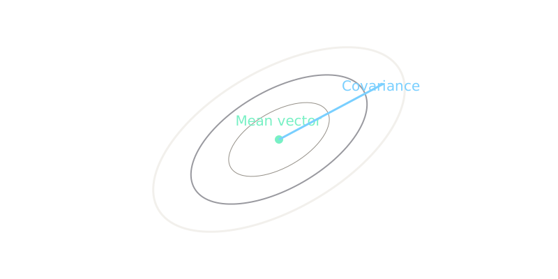
Take a round archery target: concentric circles around a bullseye, with rings marking one, two and three standard deviations. Now stretch the rubber sheet wider in one direction than the other, then twist it 45 degrees and pin it down. The circles become tilted ellipses, but the bullseye stays the bullseye and the rings still mark the same probabilities.

The bullseye is the mean vector $\mu$ : where the cloud centers. The stretch plus twist is the covariance matrix $\Sigma$ : variances set how far each axis stretches, covariance sets the twist. A point on the first ellipse is one Mahalanobis unit out no matter which direction it lies in, exactly as every point on the original first circle was one standard deviation out.

The analogy stops where shape stops. Rubber stretches a circle into exactly one ellipse family, and the Gaussian likewise produces only ellipses. Real data forms bananas, rings and separate clusters that no amount of stretching a circle will match. When the contours need more than one center, reach for a mixture, not a bigger ellipse.

How It Actually Works

Write the density for $x \in \mathbb{R}^d$ with mean vector $\mu \in \mathbb{R}^d$ and covariance matrix $\Sigma \in \mathbb{R}^{d \times d}$ :

\mathcal{N}(x \mid \mu, \Sigma) = \frac{1}{(2\pi)^{d/2}\sqrt{\det \Sigma}} \exp\left(-\tfrac{1}{2}(x - \mu)^\top \Sigma^{-1}(x - \mu)\right)

In plain words: $\mu$ is the center of the cloud, $\Sigma$ is its shape and tilt, $\det \Sigma$ sets the normalizing volume, and the exponent measures squared distance in the curved ruler $\Sigma$ defines. Every symbol is used below, none is decorative.

Three readings of $\Sigma$ that practitioners actually use:

Variances on the diagonal $\Sigma_{ii}$ set the spread along each axis. Standard deviations are their square roots.
Covariances off the diagonal $\Sigma_{ij}$ set the tilt. Divided by both standard deviations they become correlations in $[-1, 1]$ , which speak strength instead of units.
Eigen-structure sets the ellipse axes. The eigenvectors of $\Sigma$ point along the ellipse axes and the square roots of the eigenvalues are the half-lengths of the 1-sigma contour.

The exponent has its own name because it is used constantly. The Mahalanobis distance is $D_M(x) = \sqrt{(x - \mu)^\top \Sigma^{-1}(x - \mu)}$ : Euclidean distance after whitening by $\Sigma$ . Contours of equal density are contours of equal Mahalanobis distance, which is why the diagram draws ellipses and labels one of them $M = 1$ .

Worked example

Take $d = 2$ with $\mu = [0, 0]$ and $\Sigma = [[5, 3], [3, 5]]$ .

Variances are $5$ and $5$ , so each standard deviation is $\sqrt{5} \approx 2.236$ . Covariance $3$ divided by $5$ gives correlation $0.6$ : a clear rising tilt. Determinant $\det \Sigma = 25 - 9 = 16$ , so $\sqrt{\det \Sigma} = 4$ and the inverse is $\frac{1}{16}[[5, -3], [-3, 5]]$ . Eigenvalues are $8$ and $2$ since the trace is $10$ and $(10 \pm \sqrt{100 - 64})/2 = 8, 2$ , so the 1-sigma ellipse has half-lengths $\sqrt{8} \approx 2.828$ along $(1, 1)$ and $\sqrt{2} \approx 1.414$ along $(1, -1)$ : a 45-degree tilt, exactly as drawn.

Test the point $x = (2, 2)$ with displacement $dx = [2, 2]$ :

D_M^2 = \tfrac{1}{16}(5 \times 4 + 5 \times 4 - 2 \times 3 \times 2 \times 2) = \tfrac{1}{16}(20 + 20 - 24) = 1

so $D_M = 1$ : the point sits exactly on the 1-sigma contour, which is why the diagram places it at the tip of the major axis. Its density is $1/(8\pi) \times e^{-0.5} \approx 0.6065 / 25.1327 \approx 0.0241$ .

Marginals and conditionals fall out without integration. Each marginal is Gaussian: $X_1 \sim \mathcal{N}(0, 5)$ and $X_2 \sim \mathcal{N}(0, 5)$ . Given $X_1 = 2$ , the conditional is $X_2 \mid X_1 = 2 \sim \mathcal{N}(1.2, 3.2)$ , since the conditional mean is $(3/5) \times 2 = 1.2$ and the conditional variance is $5 - 9/5 = 16/5 = 3.2$ . Conditioning shrinks the variance from $5$ to $3.2$ because part of $X_2$ is explained by $X_1$ .

Code

The snippet evaluates the worked fixture directly: squared Mahalanobis distance and density at $(2, 2)$ , with no library beyond NumPy.

1import numpy as np2
3mu = np.array([0.0, 0.0])4Sigma = np.array([[5.0, 3.0], [3.0, 5.0]])5x = np.array([2.0, 2.0])6
7dx = x - mu8inv = np.linalg.inv(Sigma)9m2 = float(dx @ inv @ dx)10dens = float(np.exp(-0.5 * m2) / (2 * np.pi * np.sqrt(np.linalg.det(Sigma))))11
12print(round(m2, 4))    # -> 1.013print(round(dens, 4))  # -> 0.0241

One and $0.0241$ , matching the hand calculation. The dx @ inv @ dx line is the Mahalanobis form; everything else is the normalizer.

Watch Out For

Fitting one Gaussian to data with two centers

A single Gaussian has one $\mu$ , so on bimodal data the fitted mean lands between the clusters where no data lives. The classic case is two well-separated blobs: the maximum-likelihood center sits in the empty middle, the covariance inflates to cover both, and the density peaks exactly where the data is absent. Samples from the fit then look nothing like the training set, and downstream thresholds built from the contours misfire.

The symptom is a mean with low data density around it and residuals that cluster rather than scatter. The fix is a mixture with one component per center, or a check before fitting: if a histogram or a 2-D scatter shows two humps, do not fit one bell. The diagram's limit line states the same boundary: one Gaussian cannot fit separate clusters.

Inverting a singular or near-singular covariance

When two features are nearly perfectly correlated, rows of $\Sigma$ nearly repeat and $\det \Sigma$ approaches zero. The inverse then explodes: tiny measurement noise in $x - \mu$ multiplies into enormous Mahalanobis distances, densities swing wildly, and np.linalg.inv may warn or return garbage. Duplicated columns, one-hot groups with a dropped-category bug, or more dimensions than samples all create this.

The symptom is a determinant near zero, a condition number in the millions, or Mahalanobis distances that change drastically when one sample is removed. The fixes in order: remove the duplicated feature, add a small jitter to the diagonal ( $\Sigma + 10^{-6}I$ ), or work with the pseudo-inverse and a rank check. Never trust a density whose normalizer divides by a near-zero determinant.

The Quick Version

The multivariate Gaussian is the joint law fully described by a mean vector $\mu$ and a covariance matrix $\Sigma$ .
Diagonal entries of $\Sigma$ set axis spreads; off-diagonals set tilt; correlation rescales tilt into $[-1, 1]$ .
Contours of equal density are ellipses of equal Mahalanobis distance $D_M = \sqrt{(x-\mu)^\top \Sigma^{-1}(x-\mu)}$ .
With $\Sigma = [[5, 3], [3, 5]]$ , correlation is $0.6$ , the determinant is $16$ , and $(2, 2)$ sits exactly at $D_M = 1$ with density about $0.0241$ .
Marginals and conditionals of a Gaussian are Gaussian, with conditioning shrinking variance, here from $5$ to $3.2$ .
One Gaussian cannot fit separate clusters, and a near-singular $\Sigma$ breaks the inverse, so check modality and the determinant before trusting a fit.