Natural Gradient

The natural gradient rescales updates by the Fisher information, so steps are measured in model behavior change rather than raw parameter distance.

Fisher rescaling turns a skewed parameter step into an even move in distribution space

Why Does This Exist?

Plain gradient descent measures distance in parameter coordinates. Reparametrize the model (say, scaling one weight by 100 and dividing the next layer) and the same behavior change looks 100 times larger, so the optimizer takes a different path to the same place. That coordinate dependence wastes steps whenever parameters have mismatched scales, which is nearly always in deep networks.

The natural gradient fixes the ruler. It defines distance between models by KL divergence of their predictive distributions, whose local curvature is the Fisher information matrix $F$ . The update $\tilde{\nabla}L = F^{-1}\nabla L$ is invariant to smooth reparametrization. Geometry view: Fisher information metric. Implementation cousin: Amari natural gradient.

The one idea you need first

KL divergence measures how much one predictive distribution differs from another. For a tiny parameter move $\delta$ , it grows quadratically as $\frac{1}{2}\delta^T F \delta$ . So $F$ is the local ruler of behavior change. Background in KL divergence.

Think of It Like This

A map with a stretched axis

Imagine a city map where the east-west axis is drawn at one mile per inch but north-south at ten miles per inch. The shortest route on paper is not the shortest drive, because the paper lies about one direction.

Plain gradient descent trusts the paper. The natural gradient carries the true scale card: it shrinks moves along the stretched axis and stretches moves along the compressed one, so each step is even in miles, not inches.

Where the analogy stops: the Fisher ruler changes at every point and must be re-estimated, while a map scale is printed once.

How It Actually Works

For a model $p(y \mid x; \theta)$ with loss $L(\theta)$ :

F(\theta) = \mathbb{E}\left[\nabla \log p \;\nabla \log p^T\right], \qquad \theta_{t+1} = \theta_t - \eta F^{-1}\nabla L

$F$ equals the expected Hessian of the negative log-likelihood under the model, so this is a Gauss-Newton-like step using behavior curvature instead of loss curvature. Exact inversion costs $O(n^3)$ , so practice uses diagonal, block-diagonal (K-FAC), or Hessian-free approximations. The geometric sequel is statistical manifolds.

Worked example

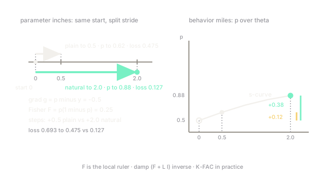
Bernoulli model with $p = \sigma(\theta) = 1/(1+e^{-\theta})$ , single observation $y = 1$ , at $\theta = 0$ ( $p = 0.5$ ):

Loss (negative log-likelihood): $-\log 0.5 \approx 0.693$ . Gradient: $p - y = -0.5$ .
Fisher: $p(1-p) = 0.25$ . Plain step with $\eta = 1$ : $\theta \to 0.5$ .
Natural step: $F^{-1}\nabla L = (-0.5)/0.25 = -2$ , so $\theta \to 0 - 1 \times (-2) = 2.0$ . New $p = \sigma(2) \approx 0.881$ , loss $-\log 0.881 \approx 0.127$ .
Plain gradient cut loss to $-\log \sigma(0.5) \approx 0.475$ . The natural step moved five times further in probability (0.38 vs 0.12 gain) because it knew the parameter was in a flat-probability zone.

Code

1import numpy as np2
3
4def sigmoid(t: float) -> float:5    return 1.0 / (1.0 + np.exp(-t))6
7
8theta, y, eta = 0.0, 1.0, 1.09p = sigmoid(theta)10g = p - y            # plain gradient of NLL11F = p * (1 - p)      # Fisher for Bernoulli12print(round(-np.log(p), 3))              # -> 0.69313print(round(theta - eta * g, 3))         # -> 0.5 plain update14print(round(theta - eta * g / F, 3))     # -> 2.0 natural update

Watch Out For

Inverting a singular empirical Fisher

With small batches the empirical Fisher is rank-deficient and its inverse explodes along unobserved directions. Updates shoot to huge values and loss goes to NaN.

Always damp: solve $(F + \lambda I)^{-1}g$ with $\lambda$ around $10^{-3}$ times the Fisher trace, and verify the update norm before applying it.

Paying full Fisher cost on every step

Exact Fisher inversion on a million parameters is hopeless. Teams that try stall training with hours-long steps.

Use K-FAC, diagonal, or update the curvature estimate every 10 to 100 steps instead of every step. The curvature changes slower than the gradient.

The Quick Version

Plain gradients depend on parametrization; the natural gradient uses behavior distance instead.
The Fisher matrix is the local ruler from KL divergence curvature.
The update is inverse-Fisher times gradient, with damping to handle singularity.
Exact inversion is cubic cost, so K-FAC and diagonal approximations carry practice.
Reparametrizing the model leaves the natural path unchanged.